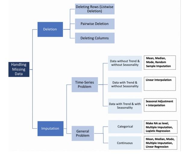
Handling Missing Values

2018-10-18 22:08

Harun

Source

Tags:

In this notebook we summarize the methods to deal with missing values
Missing values can happen because of human error, machine sensor malfunction, database failures, etc
Missing values can reduce the predictive power and lead to biased results if not handled properly.
There are different solutions for data imputation depending on the kind of the problem like time series analysis, regression etc.

tooth

Types of Missing Values¶

Understanding the reasons why data are missing is important for handling the remaining data correctly.
We need to understand patterns and randomness of missingness.
If values are missing completely at random, the data sample is likely still representative of the population.
But if the values are missing systematically, analysis may be biased.

Missing Completely at Random :

The missing data are just a random subset of the data.
So, there are no systematic differences between the missing and non-missing values.
The missing and non-missing values will have similar distributions.
For instance, if data are missing because a researcher dropped the test tubes or survey participants accidentally skipped questions are likely to be Missing Completely at Random.

Missing at Random

Firstly, this name is confusing
Missing at random means there might be systematic differences between the missing and non-missing values, but these can be entirely explained by other non-missing features.
A better name would actually be Missing Conditionally at Random, because the missingness is conditional on another feature(s).
For example, if blood pressure data are missing at random, CONDITIONAL on age and sex, then the distributions of missing and non-missing blood pressures will be similar among people of the same age and sex.

For better understanding the difference between Missing Completely at Random and Missing at Random

Missing NOT at Random (Missing with bias):

The value of the feature that's missing is related to the reason it's missing
It commonly occurs when people do not want to reveal something very personal or unpopular about themselves. For instance:
- People with high salaries generally do not want to reveal their incomes in surveys or
- Let’s assume that females generally do not want to reveal their ages!

In this case, the missing data mechanism for income is non-ignorable.
Whether income is missing or non-missing is related to its value, not random.

Effects of Randomness of Missing Data

If data are missing not randomly, dropping missing samples and only using complete samples for analysis can give highly biased results. For example,
- Taking into account the income data, if proportionally more low and moderate income individuals are left in the sample because high income people are missing, an estimate of the mean income will be lower than the actual population mean.

So we have to be really careful before removing observations because systematic biases in data deleted may produce systematic biases in data retained

imputation

How can we understand if a data is missing at random?¶

A technique is to create dummy variables for whether a feature which has missing values

1 = missing
0 = observed
We can then run t-tests and chi-square tests between this feature and others in the data set to see if the missingness on this feature is related to the values of others.
For example, if women really are less likely to tell you their weight than men, a chi-square test will tell you that the percentage of missing data on the weight variable is higher for women than men.

Handling Missing Data¶

Detecting Missing Values by Pandas¶

pandas provides the isna() and .notna() functions to detect the missing values
They are also methods on Series and DataFrame objects
We can use pd.isna(df) or df.isna() versions

.isna() can detect NaN type of missing values however missing values can be in different forms like "n/a", "na", "--"
A way dealing this problem is introducing different formats as missing values to pandas during import.

Here’s an example of how we would do that:
- Make a list of different missing value formats
- missing_values = ["n/a", "na", "--"]
- Pass the list in the na_values parameter
- df = pd.read_csv("property data.csv", na_values = missing_values)

During import pandas will convert those values into NaN and recognize when them as missing values with function calls
You might not be able to catch all of different missing value types right away.
As you work through the data and see other types of missing values, you can add them to the list.
If you count the number of missing values before converting these non-standard types, you could end up missing a lot of missing values.

Unexpected Missing Values¶

We can classify the values that are irrelevant as unexpected missing values
For example if our feature is expected to be a categorical(string, 'Yes' or 'No), but there’s a numeric value (say '15'), then technically this is also a missing value.
We need to think through a strategy for detecting these types of missing values.
Here’s a solution for our example:
- Loop through the column with unexpected missing values
- Try and turn the input into an integer.
- If the entry can be changed into an integer, replaced it with NaN
- If the number can’t be an integer, we know it’s a string, so keep going

Let’s take a look at the code and then we’ll go through it in detail:

In [ ]:

# Detecting numeric values in a categorical column
cnt=0
for row in df['col_with_unexpected_mv']:
    try:
        # try and change the entry to an integer using int(row)
        int(row)
        # If the value can be converted to an integer, replace to a missing value using Numpy’s np.nan
        df.loc[cnt, 'col_with_unexpected_mv']=np.nan # We can use .iloc() if the index is not a range index
    except ValueError:
        # if it can’t be converted to an integer, we pass and keep going
        pass
    cnt+=1

to find the missing value percentage of any col, say col5:
- df['col5'].isna.sum()/len(df)

Deletion¶

Deleting Samples

Deletion of any sample if that sample has missing data on any feature
- can substantially lower the data size
- can also lead to biased results if the missing data is not missing at random
- works when there are sufficient data, even though you lost part of your data set and
- when the missing data are Missing Completely at Random.
- can be useful when most values in a column are missing.

Still we should first look for the other solutions.

Deleting Rows With Missing Values

missing_samples= df.isna().any() (finds the rows with missing values)
df[missing_samples].dropna(inplace=True) (deletes the values with missing values)

or directly subset the non-missing values

df= df[df.notna()]

We can keep only ROWs where particular features are NOT null

df_no_missing = df[df["col1"].notna() & df["col4"].notna() & df["col6"].notna()]

Deleting Features With Missing Values

We can think of dropping the features which have 60% of the samples missing but only if that variable is insignificant.
Still we should evaluate well if we could use those features by imputation

In python deleting columns:

del df.column_name
df.drop('column_name', axis=1, inplace=True)

Imputation¶

Deleting the entire rows and/or columns with missing values may cause losing valuable data.
A better strategy is to impute the missing values, i.e., fill with the values by infering them from the known part of the data.
Imputing does not always improve the predictions, so we need to check the performance of models via cross-validation after imputing
Sometimes dropping rows or using marker values might be more effective.

There are many options we could consider when replacing a missing value, for example:
- A constant value that has meaning within the domain, such as 0, distinct from all other values.
- A value from another randomly selected record.
- A mean, median or mode value for the column.
- A value estimated by another predictive model.

Filling in the missing values with the mean of the features raduces variance in the dataset since we replace unknown values with the central value and produces bias results.
The median is a more robust estimator for data with high magnitude features which could dominate results (known as a ‘long tail’).

When choosing the imputation methods we neeed to take into account if the dataset is a timeseries or not

Time-Series And Missing Values¶

Time series may not be linear like the temperature over the year. It follows more like a sinusoidal motion, the value is affected by many factors:
- seasonality,
- trend,
- other random factors.

We should take into account if there is a trend and seasonality in our timeseries when imputing
Replacing the missing values with the mean, median or mode ignores the time series characteristics or relationship between the features.

Filling Methods with Pandas¶

fillna() can “fill in” missing values in a couple of ways:

For example, we can use fillna() to replace missing values with the mean value for each column, as follows:
- df.fillna(df.mean(), inplace=True)

Replace NA with a scalar value or a string:
- df.fillna(0), df.fillna("missing")

Fill the gaps forward or backward: Using the filling arguments, we can propagate non-NA values forward or backward:
- df.fillna(method='pad') , df.fillna(method='ffill') fill values forward
- df.fillna(method='backfill') bfill / backfill fills values backward
- ffill() is equivalent to fillna(method='ffill') and
- bfill() is equivalent to fillna(method='bfill')

Imputation With Sklearn¶

Missing values in the data is incompatible with scikit-learn estimators which assume that all values in an array are numerical
We can use Sklearn imputing objects by fit and transform methods
One advantage of Sklearn imputers is that we can use them in pipelines

from sklearn.impute import SimpleImputer
imp = SimpleImputer(missing_values=np.nan, strategy='mean')
imp.fit(X)
imp.transform(X)
or we can use imp.fit_transform(X) instead of seperate fit and transform

Marking imputed values¶

The MissingIndicator transformer of Sklearn is useful to transform a dataset into corresponding binary matrix indicating the presence of missing values in the dataset.
This transformation is useful in conjunction with imputation.
When using imputation, preserving the information about which values had been missing can be informative.
NaN is usually used as the placeholder for missing values however, it enforces the data type to be float.
The parameter missing_values allows to specify other placeholder such as integer.
When using the MissingIndicator in a Pipeline, be sure to use the FeatureUnion or ColumnTransformer to add the indicator features to the regular features.

from sklearn.impute import MissingIndicator
indicator = MissingIndicator(missing_values= -1) # Missing values are marked as -1
mask_missing_values_only = indicator.fit_transform(X)

Interpolation¶

Interpolation means using the known (pre-existing) data to infer the values of missing data by using the values on either side of a gap in the data.
Pandas provides a nice selection of simple and more complex interpolation methods. With domain knowledge we can choose which methods to use.

Here are the methods:

‘linear’: Ignore the index and treat the values as equally spaced.
‘time’: Works on daily and higher resolution data to interpolate given length of interval.
‘index’, ‘values’: use the actual numerical values of the index.
‘pad’: Fill in NaNs using existing values.

‘nearest’, ‘zero’, ‘slinear’, ‘quadratic’, ‘cubic’, ‘spline’, ‘barycentric’, ‘polynomial’: Passed to scipy.interpolate.interp1d.
‘krogh’, ‘piecewise_polynomial’, ‘spline’, ‘pchip’, ‘akima’: Wrappers around the SciPy interpolation methods of similar names.
‘from_derivatives’: Refers to scipy.interpolate.BPoly.from_derivatives
For the details of this methods you can check the Scipy tutorial page and the reference guides pages for interpolation

Examples:

df.interpolate(method='zero')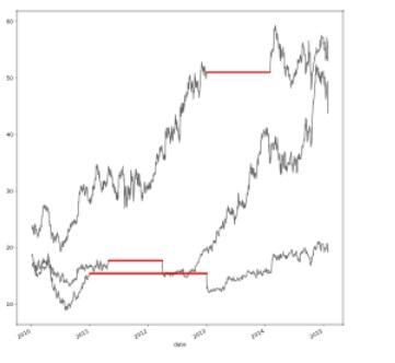

Interpolate linearly
df.interpolate(method='linear')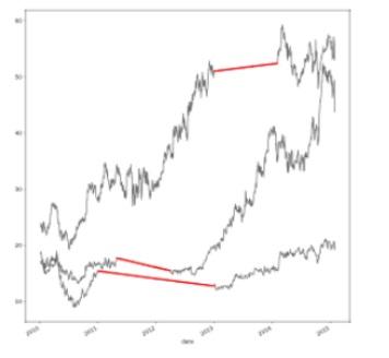

Interpolate with a quadratic function
df.interpolate(method='quadratic')

As we can see, the method we use for interpolation has a big effect on the outcome.
For example, linear Interpolation works well for a time series with some trend but is not suitable for seasonal data

Template for Interpolation¶

Since we have the many option to fill-in missing values we can use this tamplate to make an fill-in function. Here we will utilize the .interpolate() and .fillna() method in the function

In [ ]:

def fill_missing(fill_method='linear', order=2):
    
   # Use interpolation with "spline" and "polynomial" methods. They need order argument
    if algorithm in ['spline', 'polynomial'] :
        df = df.interpolate(method=fill_method, order=order)
    # Use fillna method  
    elif algorithm in ['ffill', 'bfill']:
        df = df.fillna(method=fill_ method)
    else:
        # Use interpolate methods without order argument
        df = df.interpolate(method=fill_method)
        
    return df

Plot Data Filled With Different Methods¶

We can see the outcomes of the fill methods by plotting them on one chart. Here is the template:

In [ ]:

# Create a figure and axes
fig, ax = plt.subplots()

# List all the methods to be used for filling-in
fill_methods = ['linear', 'quadratic', 'cubic', 'spline', 'polynomial', 'pchip', 'ffill', 'bfill']

# Loop over the methods
for method in fill_methods:
    # Pass in the method in the function fill_missing
    new_df = fill_missing(fill_method='linear', order=2)]
    ax = new_df['ColumnToPlot'].plot()

handles, not_needed = ax.get_legend_handles_labels()
ax.legend(handles, fill_methods, loc='best')

plt.show()

Adding Dummy Variables¶

Sometimes missing values are informative and weren't generated randomly.
If they’re not at random, the fact that a value is missing is itself information and can be expressed as extra binary features.
It's a good practice to add binary features (create a binary flag: missing (1) or not missing (0)) to check if there is missing values in each row for each feature that has missing values.
For example, "feature3" column has missing values, so we can add a feature "feature3_missing" which takes the values ∈{0,1}.

While the dummy variable adjustment method is not a proper way when data are truly missing (missing at random), it may still be appropriate in examples like:
- If someone is not sharing her contact info (missing) it could mean that she is not open to being contacted
- Married respondents may be asked to rate the quality of their marriage, but that question has no meaning for unmarried respondents.
- you might have questions about mother’s education and father’s education, but the father is unknown or was never part of the family.
- you might have spouse’s education, but there is no spouse.
Afterwards we will check if the the added binary features improve the model or not.
If there is not improvement we can conclude that the features with missing values does not have a pattern
One disadvantage is if we have many features with missing values it will inflate our feature space drastically
Here's how it might look:

In [ ]:

# make copy to avoid changing original data (when Imputing)
new_df= original_df.copy()

# Get the columns with missing values
cols_with_missing = (col for col in new_df.columns 
                                 if new_data[col].isnull().any())

# Create new binary columns from the columns with missing values
for col in cols_with_missing:
    new_df[col + '_was_missing'] = new_df[col].isnull()

# Keep the column names
column_names=new_df.columns

# Impute the dataframe 'new_data' with SimpleImputer from Sklearn
my_imputer = SimpleImputer()
new_df = pd.DataFrame(my_imputer.fit_transform(new_df.values))

# Add the column names of the original data
new_df.columns = column_names

In some cases this approach will meaningfully improve results. In other cases, it doesn't help at all.

We need to compare the scores of the models by using:
- a dataset whoose missing values are dropped
- a dataset whoose missing values imputed
- a dataset with extra columns showing what was imputed

Score of the Dataset with Dropped Missing Values¶

We can use a template like this get the score from dropped values

In [ ]:

# List the column names with missing values in X_train
cols_with_missing = [col for col in X_train.columns if X_train[col].isnull().any()]

# Drop the columns with missing values from X_train
reduced_X_train = X_train.drop(cols_with_missing, axis=1)

# Drop the columns with missing values from X_test
reduced_X_test  = X_test.drop(cols_with_missing, axis=1)

# Get the score from reduced dataset
print(score(reduced_X_train, reduced_X_test, y_train, y_test))

Score of the Dataset with Imputed Values¶

We can use a template like this get the score from imputed values

In [ ]:

from sklearn.impute import SimpleImputer

# Instantiate the SimpleImputer
my_imputer = SimpleImputer()

# Fit the imputer on the X_train dataset and transform it
imputed_X_train = my_imputer.fit_transform(X_train)

# Transform the X_test
imputed_X_test = my_imputer.transform(X_test)

# Get the score from imputed dataset
print(score(imputed_X_train, imputed_X_test, y_train, y_test))

Score of the imputed dataset with Extra Columns Showing What Was Imputed¶

In [ ]:

# Copy the X_train dataset
imputed_X_train_plus = X_train.copy()

# Copy the X_test dataset
imputed_X_test_plus = X_test.copy()

# Get the column names from the X_train with missing values
cols_with_missing = (col for col in X_train.columns 
                                 if X_train[col].isnull().any())

# Create new binary columns from the columns with missing values for X_train and X_test
for col in cols_with_missing:
    imputed_X_train_plus[col + '_was_missing'] = imputed_X_train_plus[col].isnull()
    imputed_X_test_plus[col + '_was_missing'] = imputed_X_test_plus[col].isnull()
    

# Imputate with SimpleImputer
my_imputer = SimpleImputer()

# Fit the imputer on the X_train dataset and transform it
imputed_X_train_plus = my_imputer.fit_transform(imputed_X_train_plus)

# Transform the X_test
imputed_X_test_plus = my_imputer.transform(imputed_X_test_plus)

# Get the score from imputed dataset
print(score_dataset(imputed_X_train_plus, imputed_X_test_plus, y_train, y_test))

Imputating Using Regression¶

This method assumes the linear relationship between features.
It assumes that the value of one features changes in a linear way with the other features.
The missing values are replaced by a linear regression function instead of replacing all missing data with a statistics.
But in most of the cases, the relationship is not linear and using regression imputation in such cases will bias the model.
We can use the statsmodel's regression imputation

Imputing using K-Nearest Neighbors¶

We compute distance between all examples (excluding missing values) in the data set and take the average of k-nearest neighbors of each missing value based on some distance measure and number of nearest neighbors.

There's no implementation for it yet in sklearn and it's pretty inefficient to compute it since we'll have to go through all examples to calculate distances.

One of the most attractive features of the KNN algorithm is that it is simple to understand and easy to implement.
One of the obvious drawbacks of the KNN algorithm is that it becomes time-consuming when analyzing large datasets because it searches for similar instances through the entire dataset.

Furthermore, the accuracy of KNN can be severely degraded with high-dimensional(curse of dimensionality) data because there is little difference between the nearest and farthest neighbor.

Multiple Imputation¶

Instead of substituting missing value with a single value like mean, imputing by a set of values that better represent each missing value is a smarter idea
In Multiple Imputation method, for all features having missing values the process is repeated multiple times as the name itself suggests
Multiple imputation follows 3 stages: imputation, analysis and pooling
At the moment MICE can't be used as a transformer in Sklearn pipelines but probably we will be able to use with the next version. Here is the open issue page

Steps:¶

Imputation:

In this step, N imputed datasets are generated from a distribution which results in N complete data sets.
The distribution can be different for each missing entry.
The result is N imputed datasets.

Analysis

Analyze each of N completed dataset through pipeline (e.g. feature engineering, clustering, regression, classification).
Each estimates will differ slightly because the data differs slightly.
The N final analysis results (e.g. held-out validation errors) allows us to understand how analytic results may differ as a consequence of the inherent uncertainty caused by the missing values.

Pooling

The output obtained after data analysis is pooled to get the final result using simple rules.
Combine results, calculating the variation in parameter estimates.
However, multiple imputation is not always quick or easy. It requires:
- that the missing data is missing randomly
- a very good imputation model
- knowing your data very well and having features that will predict missing values.

Imputation of Train-Test Set and Data Leakage¶

Should imputation take place before splitting the dataset or after splitting?
If we should impute the train dataset after splitting , how should the validation, test split be imputed?
There is an interesting discussion on Kaggle Questions and Answers about the possibility of data leakage stemming from imputing

Sources:
https://scikit-learn.org/stable/modules/impute.html#impute
https://towardsdatascience.com/how-to-handle-missing-data-8646b18db0d4
https://www.theanalysisfactor.com/mar-and-mcar-missing-data/
https://www3.nd.edu/~rwilliam/stats2/l12.pdf
https://www.ncbi.nlm.nih.gov/pmc/articles/PMC3668100/
https://stats.stackexchange.com/questions/358443/handling-nas-in-a-regression-data-flags
https://stats.stackexchange.com/questions/144924/missing-data-and-imputation-in-general
http://www.indjst.org/index.php/indjst/article/viewFile/110646/80197
https://towardsdatascience.com/data-cleaning-with-python-and-pandas-detecting-missing-values-3e9c6ebcf78b
https://www.kaggle.com/dansbecker/handling-missing-values
http://jmlr.csail.mit.edu/papers/volume8/saar-tsechansky07a/saar-tsechansky07a.pdf

Types of Missing Values¶

How can we understand if a data is missing at random?¶

Handling Missing Data¶

Detecting Missing Values by Pandas¶

Unexpected Missing Values¶

Deletion¶

Imputation¶

Time-Series And Missing Values¶

Filling Methods with Pandas¶

Imputation With Sklearn¶

Marking imputed values¶

Interpolation¶

Template for Interpolation¶

Plot Data Filled With Different Methods¶

Adding Dummy Variables¶

Score of the Dataset with Dropped Missing Values¶

Score of the Dataset with Imputed Values¶

Score of the imputed dataset with Extra Columns Showing What Was Imputed¶

Imputating Using Regression¶

Imputing using K-Nearest Neighbors¶

Multiple Imputation¶

Steps:¶

Imputation of Train-Test Set and Data Leakage¶

Comments