Metrics - Precision, Recall, F1 Score

2018-10-14 22:08

Harun

Tags:

We continue with the methods of measurement of classification models' performance
The confusion matrix is very helpful to understand the details of our classifiers performance however we still need some metrics to interpret more directly to choose the best model
So in this notebook we will talk about the metrics like sensitivity (recall), specifity, precision and F1 score
These metrics can be computed from a confusion matrix and are more efficient to choose the best model.

In the first part we remind the concepts and in the second part we will apply these concepts for evaluating some classifiers' performance
Skitlearn provides all these scores by ClassificationReport

In [1]:

# Notebook setup
import pandas as pd
import matplotlib.pyplot as plt

from sklearn.linear_model import LogisticRegression, LogisticRegressionCV, LogisticRegression, SGDClassifier
from sklearn.svm import LinearSVC, NuSVC, SVC
from sklearn.neighbors import KNeighborsClassifier
from sklearn.ensemble import BaggingClassifier, ExtraTreesClassifier, RandomForestClassifier

from sklearn.model_selection import train_test_split
from sklearn.pipeline import Pipeline
from sklearn.metrics import f1_score, precision_score, recall_score

import category_encoders as ce
from yellowbrick.classifier import ClassificationReport

import warnings 
warnings.filterwarnings("ignore")
%matplotlib inline

Part-1¶

Accuracy, Sensitivity (Recall), Specifity, Precision¶

Lets talk about these metrics
In this contex POSITIVE means that an instance belonging to the class of interest

Accuracy¶

Overall how often the classifier is predicting correctly Positive Class (1) and the Negative Class(0)
#all correct predictions (diagonal values) / #all predictions

With imbalance datasets the accuracy is not a good metric.

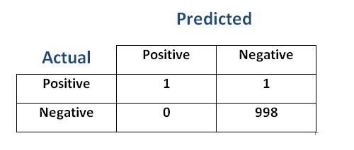
Look at the confusion matrix below

We have 998 NEGATIVE and 2 POSITIVE classes.
The accuracy 999/1000=0.999. It is a high accuracy score
However accuracy by itself is not reliable in this case.
Think of a classifier which allways only says NEGATIVE when predicting any sample, also get a 998/1000= 0.998 accuracy
Accuracy can be largely contributed by a large number of TRUE(ly) predicted NEGATIVEs (like non-spam, non-fradulent, not sick etc) which in most business circumstances, we do not focus on much.

acc1

True Positive Rate (Sensitivity, Recall)¶

The ability of a classifier to find all POSITIVE instances.
How good is the model at capturing the Positive Class samples

Among all of the actual Positive Class(1) samples, what portion of them is classified correctly?

#samples TRUE(ly) predicted POSITIVE / #all actual POSITIVE samples

The term "recall" is coming from information retrivieal domain.
Here you can find an explanation on the semantic of the term
It may have been better to use Recall Rate term

If we compute the sensitivity of the table above, we will see that it is not high even though accuracy is very high.
- True Positive= 1
- All Positives= 2
- True Positive Rate = 1/2 -> 0.5

all3

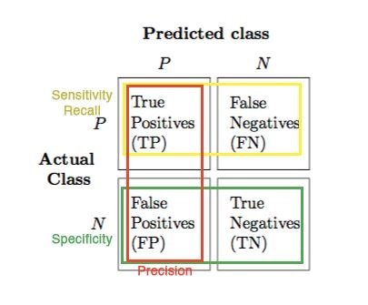
True Negative Rate (Specifity)¶

The ability of a classifier to find all NEGATIVE instances.
How good is the model at capturing the NEGATIVE Class samples

Among all of the Negative Class(0) samples, what portion of them is predicted correctly?
#samples TRUE(ly) predicted NEGATIVE / #all NEGATIVE samples

An Analogy for `Sensivity` and `Specifity`¶

Think of a drug-sniffing security dog.

If the dog’s nose is perfectly sensitive to the smell of drugs, then it will detect all the hidden packets of drugs;
if it is less sensitive, then it will fail to detect some of the packets.

At the same time, the dog should react specifically to drugs, and not for food or other objects

If the dog is highly specific in its reactions, it will only react to drugs;
if it is less specific, then it will react to other stuff also

We expect from the dog to

higly detect the bags with drugs (find all actual POSITIVEs)
higly NOT to detect the bags without drugs, let them go without any reaction, (find all the actual NEGATIVEs)

So there is a trade off between Specificity (True Positive Rate) and Sensitivity (True Negative Rate).

If the dog treat every bag as drug contained;
- this procedure is perfectly sensitive (perfect True Positive Rate)
- it will detect every packet of drugs, all actual POSITIVEs for sure but
- not specific at all. It creates cost of false accusations.

If the dog treat all the bags as none of them containing drugs
- this is perfectly specific (perfect True Negative Rate)
- it means it will find all actual NEGATIVEs and not react to them. (We will never make a false accusation), but
- not sensitive at all. It creates cost of missing the drug contained bags

False Positive Rate¶

Among all of the Negative Class(0) samples, what is the fraction of the predictions that the model falsely predict as POSITIVE?
#samples FALSE(ly) predicted as POSITIVE / #all NEGATIVE samples

Precision¶

For all instances classified as POSITIVE Class(1), what percent was correct?
The ability of a classifer NOT to label an instance POSITIVE that is actually NEGATIVE.
#samples TRUE(ly) predicted as POSITIVE / #all predictions made as POSITIVE Class(1)

Here the denominator is the predictions, not the actual number of classes like in sensitivity and specifity
When the data is imbalanced ie has "skewed classes", precision standalone is not a good performance metric.

acc1

In the table above, again we have a skewed classes data: 998 Negative, 2 Positive

precision = TP/all POSITIVE Class(1) predictions -> 1/1 = %100
This is not relaible by itself.
Think of any classifier which allways only says POSITIVE when predicting any sample, could get the same precision

That is why we should use the Precision and Recall together for more accurate measurements
An ideal algorithm should have high precision and recall (True Positive Rate) values.
But for a given algorithm, there is a trade of between precision and recall.
Setting the classification threshold higher or lower will change the values of precision and recall

F1 Score¶

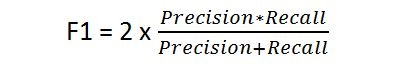
A weighted harmonic mean of precision and recall
Best score is 1.0 when both precision and recall are 1 and the worst is 0.0
When either recall or precision is small, the score will be small.

It is a convenient single score to characterize overall accuracy, especially for comparing the performance of different classifiers.

As a rule of thumb, the weighted average of F1 should be used to compare classifier models

Using $ F_1$ to compare classifiers assumes that precision and recall are equally important for the application.

If one criterion is more important than the other, then one can also use the weighted geometric mean:
- $\displaystyle F_\alpha = (1 + \alpha)($precision$\displaystyle \times$ recall$\displaystyle )/(\alpha$ precision + recall$\displaystyle ) $
- $ \alpha$ describes how much more important recall is than precision:
- use $ F_2$ if recall is twice as important as precision,
- $ F_{0.5}$ if precision is twice as important as recall.

It is still better to have separate target goals for precision and recall that a candidate classifier must meet.

Choosing a Metric for Model Evaluation¶

Choise of metric depends on our business objectives, in other words depends of what business challenge we are trying to solve using the model.

Ultimately we

make a value judgement about which errors to minimize and
choose an appropriate metric to match that judgement

Here are two different examples of problems we want to solve:

1- Email Spam Detection:
If our goal is to create a spam filter (in this case spam is POSITIVE, non-spam is NEGATIVE class):

We have to make a value judgement here between the cost of false classifications
- the cost of loosing an important mail in the spam box and
- the cost of having a spam in the inbox

In email spam detection, Precision or Specifity becomes more important as a metric because
- FALSE(ly) predicted NEGATIVEs (true spam goes into the inbox, spam not caught) is more accaptable than
- FALSE(ly) predicted POSITIVEs (non-spam goes into the spam box, normal mail caught as spam)

Precision is a good measure to determine, when the costs of FALSE POSITIVE is high.
- In email spam detection, again a FALSE POSITIVE means that an email that is non-spam (actual negative) has been identified as spam (predicted as spam).
- The email user might lose important emails in the spam box if the precision is not high for the spam detection model.

2- Fradulent Transaction Detection:
If our goal is to create a fraud detector (in this case fraudelent transaction is POSITIVE, non-fraudelent is NEGATIVE):

We have to make a value judgement here between false classifications
- the cost of labeling a normal transaction as fraudelent and
- the cost of missing a fraudelent transaction

In Fradulent Transaction Detection, we need to optimize for Sensitivity(Recall) because
- FALSE(ly) predicted as POSITIVEs (normal transactions that are flagged as possible fraud) are more acceptable than
- FALSE(ly) predicted as NEGATIVEs (fraudelent transactions that are not detected, missed the fraud case)

Sesitivity (Recall) is a good measure to determine when there is a high cost associated with FALSE NEGATIVE,
- For instance, in fraud detection or sick patient detection
- If a fraudulent transaction (actual POSITIVE) is predicted as non-fraudulent (Predicted Negative), the consequence can be very bad for the bank.
- Similarly, if a sick patient (actual POSITIVE) goes through the test and predicted as not sick (predicted as NEGATIVE), the cost associated with FALSE NEGATIVE will be extremely high if the sickness is contagious or severe

FALSE NEGATIVE and FALSE POSITIVE usually has business costs (tangible & intangible). Generally speaking,
- for the False Negative the cost comes from not taking actions towards it, like not doing anything for the fraud, sick patient cases
- for the False Positive the cost comes from taking wrong actions towards it, like sending a normal mail into spam box

These are known as Type I and Type II errors also:
Type I error (“FALSE POSITIVE”) is detecting an effect that is not present (e.g. determining a mushroom is poisonous when it is in fact edible).
Type II error (“FALSE NEGATIVE”) is failing to detect an effect that is present (e.g. believing a mushroom is edible when it is in fact poisonous).

F1 SCORE can be a choise when
- you want to seek a balance between Precision and Recall and
- there is an uneven class distribution (large number of actual NEGATIVEs).

Some points to remember:¶

Classifier performance are not one-dimensional.
Different fields use different (but related) measures of accuracy.

Classifier performance depend on
- the relative cost of Type I and Type II errors, as well as
- on the proportion of positive and negative instances in the population of interest.

Part-2¶

Loading and Exploring the Dataset¶

Lets make a classification performance evaluation on the mushroom dataset
We will use a modified version of the mushroom dataset from the UCI Machine Learning Repository.
Even though these toy datasets are not very interesting anymore because of repetitive usage, here our focus is the classification metrics not other steps of data processing. So we try to get the advantage of fast implementation of this dataset

Our objective is to predict if a mushroom is poisonous or edible based on its characteristics.
The data include descriptions of samples of mushrooms
Each species was identified as definitely edible or poisonous

In [3]:

# Url of the dataset
url='https://raw.githubusercontent.com/rebeccabilbro/rebeccabilbro.github.io/master/data/agaricus-lepiota.txt'

# Column names list
column_names=['class', 'cap-shape', 'cap-surface', 'cap-color']
# Load the data
mushrooms=pd.read_csv(url, header=None, names= column_names)

mushrooms.head(3)

Out[3]:

	class	cap-shape	cap-surface	cap-color
0	edible	convex	smooth	yellow
1	edible	bell	smooth	white
2	poisonous	convex	scaly	white

Target and Features Datasets¶

In [5]:

# Create the features dataset (X) and target dataset (y)
features = ['cap-shape', 'cap-surface', 'cap-color']
target   = 'class'

X = mushrooms[features]
y = mushrooms[target]

Classifiers Dictionary¶

Now, let's create a dictionary which contains the classifiers we want to use for our classification task
Here we create the dictionary with instantiates of Sklearn estimators without hyperparameter tuning.
In reality we need to evaluate the performance of tuned classifiers.

In [15]:

# Estimators dictionary
# We can add as more classifiers to our dictionary
# This is just a sample
estimators_dct={"NuSVC": NuSVC(),
                "SVC": SVC(), 
                "Linear SVC" : LinearSVC(),
                "SGD Classifier": SGDClassifier(),
                "KNeighbors Classifier": KNeighborsClassifier(),
                "Logistic Regression CV": LogisticRegressionCV(),
                "Logistic Legression": LogisticRegression(),
                "Bagging Classifier": BaggingClassifier(),
                "Random Forest Classifier": RandomForestClassifier(n_estimators=8),
                "Extra Trees Classifier": ExtraTreesClassifier(),
                "SGD Classifier": SGDClassifier()}

model_selection function¶

Let's define a function to get the Precision, F1 and Recall Scores of a given dictionary of models (like in the upper cell) easily without repetion.

Our function will
- take X, y datasets and an estimator dictionary
- return a nested dictionary containing the Precision, F1 and Recall Scores produced by the predictions of each model in the estimators dictionary

In [126]:

def model_selection_all(X, y, estimator_dict):
    """
    Takes X_train, y_train datasets, an estimator dictionary -> 
    returns an ordered list based on the values of the F1 scores of the classifiers in the dictionary
    """
    # Split the data as train and test
    X_train, X_test, y_train, y_test= train_test_split(X, y, test_size=0.2, random_state=11)
    
    f1_dct={}
    precision_dct={}
    recall_dct={}
    
    # Loop over the estimator_dict keys to get each estimator 
    for estimator in estimator_dict.keys():
                
        # In the pipeline we use OneHotEncoder from Category Encoders
        model = Pipeline([('encoder', ce.OneHotEncoder()),
                          ('estimator', estimator_dict[estimator])])
        
        # Instantiate the classification model 
        model.fit(X_train, y_train)
        
        # Get the predictions of the model
        predicted = model.predict(X_test)

        # Compute and return the:
        # F1 scores (the harmonic mean of precision and recall)
        # Precision scores
        # Recall scores as separate dictionaries
        f1_dct[estimator]=round(f1_score(y_test, predicted, pos_label='edible'), 4)
        precision_dct[estimator]= round(precision_score(y_test, predicted, pos_label='edible'), 4)
        recall_dct[estimator]= round(recall_score(y_test, predicted, pos_label='edible'), 4)
        
    # Return the sorted list of the F1, Precision, Recall scores in descending order
    return {"Precision": sorted(precision_dct.items(), 
                                key=lambda x:x[1], 
                                reverse=True),
            
            "Recall": sorted(recall_dct.items(), 
                             key=lambda x:x[1], 
                             reverse=True),
            
            "F1": sorted(f1_dct.items(),
                         key=lambda x:x[1], 
                         reverse=True)}

In [127]:

# Call model_selection function to get the sorted f1, precision, recall scores
model_selection_all(X, y, estimators_dct)

Out[127]:

{'Precision': [('KNeighbors Classifier', 0.7855),
  ('Bagging Classifier', 0.7497),
  ('Extra Trees Classifier', 0.7177),
  ('Random Forest Classifier', 0.7166),
  ('SVC', 0.7016),
  ('Linear SVC', 0.6959),
  ('Logistic Regression CV', 0.6959),
  ('Logistic Legression', 0.6959),
  ('NuSVC', 0.6569),
  ('SGD Classifier', 0.5322)],
 'Recall': [('SGD Classifier', 0.9612),
  ('Extra Trees Classifier', 0.7506),
  ('Random Forest Classifier', 0.7376),
  ('Bagging Classifier', 0.6941),
  ('Linear SVC', 0.6624),
  ('Logistic Regression CV', 0.6624),
  ('Logistic Legression', 0.6624),
  ('SVC', 0.6612),
  ('KNeighbors Classifier', 0.56),
  ('NuSVC', 0.5518)],
 'F1': [('Extra Trees Classifier', 0.7338),
  ('Random Forest Classifier', 0.727),
  ('Bagging Classifier', 0.7208),
  ('SGD Classifier', 0.6851),
  ('SVC', 0.6808),
  ('Linear SVC', 0.6787),
  ('Logistic Regression CV', 0.6787),
  ('Logistic Legression', 0.6787),
  ('KNeighbors Classifier', 0.6538),
  ('NuSVC', 0.5997)]}

Evaluation of Mushroom Classifier¶

We have to make a value judgement here between the cost of false classifications (False Positive and False Negative)

the cost of falsely classifying a mushroom as Poisonous which is actually Edible
the cost of falsely classifiying a mushroom as Edible which is actually Poisonous

Without doubt the cost of the latter (classifiying a mushroom as Edible which is actually Poisonous) is too high. It can cause to loose our lives!
So in mushroom detection! problem we need to be very sensitive to the presion and specifitiy scores of the Edible class

So regarding the precision scores KNeighbors Classifier has the highest precision but still not enough to rely on :)
Reminder: Here we did not do hyperparameter tuning for the classifiers

Visual Model Evaluation with Mushroom Dataset¶

Now let’s display the precision, recall, and F1 scores by using Yellowbrick’s ClassificationReport visualizer
This allows us interpret easily Type I and Type II error with numerical scores as well as color-coded heatmaps

In [124]:

def model_selection_visiual(X, y, estimator_dict):
    """
    Takes X, y datasets, an estimator dictionary -> 
    returns the Classification of classifiers in the dictionary
    """
    
    # Split the data as train and test
    X_train, X_test, y_train, y_test= train_test_split(X, y, test_size=0.2, random_state=11)
    
    f1_dct={}
    
    # Loop over the estimator_dict keys to get each estimator 
    for estimator in estimator_dict.keys():
        print(estimator)
                
        # In the pipeline we use OneHotEncoder from Category Encoders
        model = Pipeline([('encoder', ce.OneHotEncoder()),
                          ('estimator', estimator_dict[estimator])])
        
        # Instantiate the classification model 
        model.fit(X_train, y_train)
        
        # Set the current ax to the first ax in the axes_lst every time after popping the first element
        _, ax=plt.subplots()
        
        # Instantiate the classification model and visualizer
        visualizer = ClassificationReport(model,
                                          ax=ax, 
                                          classes=['edible', 'poisonous'], 
                                          size=(600, 200),
                                          cmap='YlOrBr', 
                                          title= estimator)
        visualizer.score(X_test, y_test)
        
        # argument to the poof method!
        visualizer.poof()

In [125]:

model_selection_visiual(X, y, estimators_dct)

NuSVC

SVC

Linear SVC

SGD Classifier

KNeighbors Classifier

Logistic Regression CV

Logistic Legression

Bagging Classifier

Random Forest Classifier

Extra Trees Classifier

We can plot the Classification Reports n two columns

In [86]:

def model_selection_visiual(X, y, estimator_dict):
    """
    Takes X_train, y_train datasets, an estimator dictionary -> 
    returns an ordered list based on the values of the F1 scores of the classifiers in the dictionary
    """
    
       # Create a new figure to draw the classification report on
        #fig, ax = plt.subplots()
        
    row_number=int(len( estimator_dict)/2)+1
    
        # Create figure and axes
        # Fix the number of column of the figure by ncols=2 and
        # Let the row_number change by the size of the estimator dictionary
        # Delete the last empty subplots at the end
    fig, axes = plt.subplots(nrows=row_number, ncols=2,
                                 figsize=(200, 200))
                                 #sharex=True, 
                                # sharey=True)
    # Flatten the axes and convert into a list 
    # in order to be able to pop the elements one by one
    axes_lst=list(axes.flatten())
   
    # Split the data as train and test
    X_train, X_test, y_train, y_test= train_test_split(X, y, test_size=0.2, random_state=11)
    
    f1_dct={}
    
    # Loop over the estimator_dict keys to get each estimator 
    for estimator in estimator_dict.keys():
        #print(estimator)
                
        # In the pipeline we use OneHotEncoder from Category Encoders
        model = Pipeline([('encoder', ce.OneHotEncoder()),
                          ('estimator', estimator_dict[estimator])])
        
        # Instantiate the classification model 
        model.fit(X_train, y_train)
        
        # Set the current ax to the first ax in the axes_lst every time after popping the first element
        ax=axes_lst.pop(0)
        
        # Instantiate the classification model and visualizer
        visualizer = ClassificationReport(model,
                                          ax=ax, 
                                          classes=['edible', 'poisonous'], 
                                          fontsize=20, 
                                          size=(1500, 1200),
                                          cmap='YlOrBr', 
                                          title= estimator)
        visualizer.score(X_test, y_test)

    # Note that to save the figure to disk, you can specify an outpath
    # argument to the poof method!
    [ax.remove() for ax in axes_lst]
    visualizer.poof()

In [87]:

model_selection_visiual(X, y, estimators_dct)

Sources: