With this notebook we continue our analysis of bikeshare dataset.
In this part we will do machine learning steps in order to predict the bike rentals for the given Kaggle test set and submit it to the Kaggle

time

In the previous post, we prepared the dataset partially
We created new columns and dropped the outliers regarding to the "count" column
Now we start by loading the dataset and continue to prepare it before applying machine learning algorithms

Outline:¶

About Time Data
Trigonometric functions for cyclic time data transformation
Data Split
TimeSeriesSplit for the cross validation
Sklearn Pipeline
Interpratation of RSMLE metric
Creating a custom scoring function
Kaggle submission

In [1]:

# Import the necessary modules
import pandas as pd
import matplotlib.pyplot as plt
import seaborn as sns
import numpy as np

from sklearn.preprocessing import StandardScaler
from sklearn.model_selection import TimeSeriesSplit
from sklearn.linear_model import LinearRegression
from sklearn.model_selection import train_test_split
from sklearn.model_selection import cross_val_score
from sklearn.metrics import r2_score
from sklearn.metrics import mean_squared_error
from sklearn.metrics import make_scorer
from sklearn.pipeline import Pipeline

import warnings 
warnings.filterwarnings("ignore")

%matplotlib inline
sns.set()

Let's remind our dataset¶

Kaggle terms for the dataset:¶

The training set is comprised of the first 19 days of each month, while the test set comprised of the days from 20th to the end of the month for each month.
Predict the total count of bikes rented during each hour covered by the test set, using only information available prior to the rental period.

Here is the Kaggle link for the dataset

In [2]:

# Read the bike_data_inliers
bike_data=pd.read_csv("bike_data_inliers.csv", parse_dates=["datetime"], index_col="datetime")
bike_data.head(3)

Out[2]:

	season	holiday	workingday	weather	temp	atemp	humidity	windspeed	casual	registered	count	month	weekday	hour
datetime
2011-01-01 00:00:00	1	0	0	1	9.84	14.395	81	0.0	3	13	16	1	5	0
2011-01-01 01:00:00	1	0	0	1	9.02	13.635	80	0.0	8	32	40	1	5	1
2011-01-01 02:00:00	1	0	0	1	9.02	13.635	80	0.0	5	27	32	1	5	2

In [3]:

## Filter out the casual and registered columns and 
## high correlated columns "season" (correlated with "month") and "atemp" (correlated with "temp") should be omitted
## Also in the previous post we noticed that the data record in the "weather" column is not relaible
## We will also drop it
bike_data= bike_data.drop(["casual", "registered", "season", "atemp", "weather"], axis=1)
bike_data.head(3)

Out[3]:

	holiday	workingday	temp	humidity	windspeed	count	month	weekday	hour
datetime
2011-01-01 00:00:00	0	0	9.84	81	0.0	16	1	5	0
2011-01-01 01:00:00	0	0	9.02	80	0.0	40	1	5	1
2011-01-01 02:00:00	0	0	9.02	80	0.0	32	1	5	2

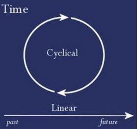
About Time Data¶

Since our data is a timeseries, i.e data recorded with a time dimension, we need to take into account the timeseries practices.

Firstly, we need to be aware of the cyclic nature of our time data

As we walked through the time frame charts in the previous post, we saw that month and hour variables are very predictive over the number of bike rentals.

This is very resaonable as we might expect that the bike usage and rentals during January is less than May due to the weather conditions and rentals at 3am in the morning is less than at 14h, during the day.

So we should use the "month" and "hour" data as features for our models. However, we have a problem of how to utilize these features.
We need to keep them numeric for the machine learning algorithms but if we use them without any transformation, it would not be so smart practice.

To make it clearer here is a question:

Which one would you expect is more similar to the bike rentals in January: rentals in December or rentals in May?

Regarding the seasonal affects we can tell that number of bike rentals in December is more similar to rentals in January, however we represent December with number 12 and May with number 5.
This is a wrong representation of the time features especially for the algorithms that use distance or the algorithms like linear regression.

As an example let's assume our model is $$ bikerentals= 15+ 2*hour $$
At 0h the number of estimated rentals = 15
At 23h the number of estimated rentals= 61
Even though there is only 1 hour difference between 0h-23h with this represantation the difference is the largest

Because of the cyclic nature of the months and hours we need to find a way of representing these features such that
- the 12th month should be closer to 1st month than 5th month or
- 23th hour should be closer to 1st hour than 7th hour.

Representation of Cyclic Time Features¶

We map each cyclical variable onto a circle such that the lowest value for that variable appears right next to the largest value.
We represent each variable with two components: x axis value and y axis value
We compute the x and y components of that point using sin and cos functions.

hours

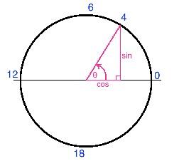
When we perform this transformation for the "month" variable, we also shift the values down by one such that it extends from 0 to 11, for convenience

NOTE: Instead of represanting the time features with trigonometric functions we can also use dummy variables. Here we will go with the trigonometric functions

In [4]:

# Create the sin and cos components of hour, month and weekday columns
bike_data['hour_sin'] = np.sin(bike_data.index.hour*(2.*np.pi/24))
bike_data['hour_cos'] = np.cos(bike_data.index.hour*(2.*np.pi/24))
bike_data['month_sin'] = np.sin((bike_data.index.month-1)*(2.*np.pi/12))
bike_data['month_cos'] = np.cos((bike_data.index.month-1)*(2.*np.pi/12))
bike_data["weekday_cos"]= np.cos((bike_data.index.weekday)*(2.*np.pi/7))
bike_data['weekday_sin'] = np.sin((bike_data.index.weekday)*(2.*np.pi/7))

# Now we can drop the columns "month", "weekday" and "hour"
bike_data=bike_data.drop(["month", "weekday", "hour"], axis=1)

Split the data¶

Even though there is a given test set (without target variable) for Kaggle submission we will analyse the data as an independent project and follow our data splitting principles
At the end we will use the Kaggle test set for submission
So, after instantiating a model we will use cross validation for evaluating model performance and hyperparameter tuning but we still we need to keep an hold-out set for our final evaluation.
Since this is a timeseries dataset we must respect to the temporal order of the data. Thus, we must use only the past data to predict the future data.
So we can take the last %5 as our hold-out data. (In the Kaggle competition the test set is the last 10 days of the months)
We need to split the data before doing transformation (incase we do) because test data points represent real-world data.
Transformation of the variables use information from the dataset like mean and standard deviation
If we transform the data before splitting we take information like mean and variance of the whole dataset thus we will be introducing future information to the training data.
Therefore, we should perform transformation over the training data. Then perform the same transformation on testing data as well, but this time using the parameters (like mean and variance) of the training data.

In [5]:

# Find the starting indice of the last five percent
last_five_percent_ind= int(len(bike_data)* 0.95)
last_five_percent_ind

# Create the hold-out dataset
hold_out_df=bike_data.reset_index().iloc[last_five_percent_ind: ,:]

print("The shape of the hold-out dataset:", hold_out_df.shape)
hold_out_df.head(3)

The shape of the hold-out dataset: (522, 13)

Out[5]:

	datetime	workingday	temp	humidity	windspeed	count	hour_sin	hour_cos	month_sin	month_cos	weekday_cos	weekday_sin
9914	2012-11-16 06:00:00	1	12.30	61	6.0032	130	1.000000	6.123234e-17	-0.866025	0.5	-0.900969	-0.433884
9915	2012-11-16 07:00:00	1	12.30	61	11.0014	367	0.965926	-2.588190e-01	-0.866025	0.5	-0.900969	-0.433884
9916	2012-11-16 09:00:00	1	13.94	53	7.0015	351	0.707107	-7.071068e-01	-0.866025	0.5	-0.900969	-0.433884

We will do training and cross validation on the rest of the data. Lets create it

In [6]:

data= bike_data.reset_index().iloc[:last_five_percent_ind, :]
data.tail(3)

Out[6]:

	datetime	workingday	temp	humidity	windspeed	count	hour_sin	hour_cos	month_sin	month_cos	weekday_cos	weekday_sin
9911	2012-11-16 03:00:00	1	12.3	65	8.9981	6	0.707107	0.707107	-0.866025	0.5	-0.900969	-0.433884
9912	2012-11-16 04:00:00	1	12.3	65	7.0015	5	0.866025	0.500000	-0.866025	0.5	-0.900969	-0.433884
9913	2012-11-16 05:00:00	1	12.3	65	6.0032	36	0.965926	0.258819	-0.866025	0.5	-0.900969	-0.433884

Features and Target Variable¶

Having splitted the hold-out dataset, now time to create the features (X) and the target (y) datasets and fit a Linear Regression model

In [7]:

# Target data
y=data["count"]

# Features data
X=data.drop(["datetime", "count"], axis=1)

In [8]:

X.head(3)

Out[8]:

	temp	humidity	hour_sin	hour_cos	month_cos	weekday_cos	weekday_sin
0	9.84	81	0.000000	1.000000	1.0	-0.222521	-0.974928
1	9.02	80	0.258819	0.965926	1.0	-0.222521	-0.974928
2	9.02	80	0.500000	0.866025	1.0	-0.222521	-0.974928

Notes about Cross Validation of Timeseries Data¶

Here is the the notes from sklearn official page :

Time series data is characterised by the correlation between observations that are near in time (autocorrelation).

However, classical cross-validation techniques such as KFold and ShuffleSplit

assume the samples are independent and identically distributed, and
would result in unreasonable correlation between training and testing instances (yielding poor estimates of generalisation error) on time series data.

Therefore, it is very important to evaluate our model for time series data on the “future” observations least like those that are used to train the model.

Time Series Split¶

TimeSeriesSplit is a variation of k-fold which

returns first k folds as train set and
the k+1 th fold as test set.

We should not shuffle our data when making predictions with timeseries.
Unlike standard cross-validation methods, successive training sets are supersets of those that come before them.
Also, it adds all surplus data to the first training partition, which is always used to train the model.

Sklearn Pipeline¶

Whenever possible, using Sklearn Pipeline object is always a smart practice because they

are powerfull tools to standardise our operations,
create an easy-to-understand workflow with clear order of steps,
are reproducable

We will create a pipeline with StandartScaler and LinearRegression objects

In [9]:

# Instantiate the pipeline with the StandardScaler and  LinearRegression
pipeline=Pipeline(steps= [("scaler", StandardScaler()),
                          ("linreg", LinearRegression())])

Cross validation scores¶

Let's use the cross_val_score from sklearn.metrics to get the scores of each split

In [10]:

# Split the timeseries data
split = TimeSeriesSplit(n_splits=5)

# Fit and score the model with cross-validation
scores = cross_val_score(pipeline, X, y, cv=split)

print("R^2 scores of each split:", scores)

R^2 scores of each split: [0.27492746 0.32817026 0.19586317 0.37070607 0.41382806]

Visualizing CV Splits for Timeseries: "TimeSeriesSplit"¶

Visualize the splits of cross validation with TimeSeriesSplit object

In [11]:

# Initialize the cross-validation iterator with 10 splits
cv = TimeSeriesSplit(n_splits=10)

fig, ax = plt.subplots(figsize=(10, 5)) 

# Loop over the cross validation splits
# cv.split() method creates train and test arrays for each split
for idx, (train, test) in enumerate(cv.split(X, y)):

    # Plot training and test indices
    indeces1 = ax.scatter(train, [idx] * len(train), c=[plt.cm.coolwarm(.1)], marker='_', lw=8)
    indeces2 = ax.scatter(test, [idx] * len(test), c=[plt.cm.coolwarm(.9)], marker='_', lw=8)
    
    ax.set(ylim=[10, -1], title='TimeSeriesSplit behavior', xlabel='Data index', ylabel='CV iterates')
    ax.legend([indeces1, indeces2], ['Training', 'Validation'])

Scoring Metric: "RMSLE"¶

Lets try to understand the metric which we will use for the Kaggle evaluation. Here is the screen shot from the Kaggle evaluation page.

scoring

So we need to take into account the metric Root Mean Squared Log Error(RMSLE) for this project. For the interpretation of RMSLE take a look to this page

RSMLE Calculator Function¶

In [12]:

# Define the RMSLE function for error calculation: rmsle_calculator
# Using the vectorized numpy functions instead of loops always better for computation
def rmsle_calculator(predicted, actual):
    assert len(predicted) == len(actual)
    return np.sqrt(
                np.mean(
                    np.power(np.log1p(predicted)-np.log1p(actual), 2)))

Custom Scoring Function¶

Having defined our function for the RMSLE calculation, now we should define a scoring function in order to use as a scoring parameter for model_selection.cross_val_score
We need this parameter for model-evaluation tools which rely on a scoring strategy when using cross-validation internally (such as model_selection.cross_val_score and model_selection.GridSearchCV)

We will use make_scorer function of Sklearn to generate a callable object (from our rsmle_calculator function) for scoring.
When defining a custom scorer via sklearn.metrics.make_scorer, the convention is that

custom functions ending in _score return a value to maximize and
for scorers ending in _loss or _error, a value is returned to be minimized.
We can use this functionality by setting the greater_is_better parameter inside make_scorer.
This parameter would be
- True for scorers where higher values are better, and
- False for scorers where lower values are better. (this will be our choise since the lower RSMLE values are better)

NOTE:

If a loss, the output of the python function, is negated by the scorer object, conforming to the cross validation convention; that scorers return higher values for better models i.e
when greater_is_better is False, the scorer object will sign-flip the outcome of the score_func.

In [13]:

# Make a custom scorer 
# rmsle_error will negate the return value of rmsle_calculator,
rmsle_error = make_scorer(rmsle_calculator, greater_is_better=False)

# Fit and score the model with cross-validation
scores = cross_val_score(pipeline, X, y, cv=split, scoring=rmsle_error)
scores

As explained the scores are negative due to the Sklearn customs. We can multiply the results by -1 for our interpretation

In [15]:

print("The cross validation scores:", scores*-1)

The cross validation scores: [1.06115722 0.97511162 1.02056734 0.93509628 0.92447915]

Hold-out Data Prediction Scores¶

In [16]:

# Hold-out target data 
y_hold=hold_out_df["count"]

# Hold-out features data
X_hold=hold_out_df.drop(["datetime", "count"], axis=1)

# Fit the pipeline to train data
pipeline.fit(X, y)

# Generate predictions for hold-out data
predictions_hold = pipeline.predict(X_hold)

# R^2 score
score = r2_score(y_hold, predictions_hold)

print("R^2 score of hold-out:", score)
print("Root mean squared error of hold-out:", np.sqrt(mean_squared_error(y_hold, predictions_hold)))
print ("RMSLE value for linear regression of hold-out: ", rmsle_calculator(y_hold , abs(predictions_hold)))

R^2 score of hold-out: 0.3889173616885714
Root mean squared error of hold-out: 120.48857034926871
RMSLE value for linear regression of hold-out:  0.715555147546642

Kaggle submission¶

Lets predict the given Kaggle test set and submit the predictions to Kaggle to get our score.
First it would be better if we combine our X and X_hold and y and y_hold datasets then train our model with more data in order to let our model learn better before predicting on a new test data i.e Kaggle test dataset which we have not yet uploaded.

In [17]:

# Combine X and X hold: combined_train
combined_X=pd.concat([X, X_hold])

# Combine the y and y hold: combined_test
combined_y =pd.concat([y, y_hold])

# Fit the model to the combined datasets
pipeline.fit(combined_X, combined_y)

Out[17]:

Pipeline(memory=None,
     steps=[('scaler', StandardScaler(copy=True, with_mean=True, with_std=True)), ('linreg', LinearRegression(copy_X=True, fit_intercept=True, n_jobs=1, normalize=False))])

In [18]:

# Read the Kaggle test data
kaggle_test=pd.read_csv("bike_kaggle_test.csv", parse_dates=["datetime"], index_col="datetime")
kaggle_test.head(3)

Out[18]:

	season	holiday	workingday	weather	temp	atemp	humidity	windspeed
datetime
2011-01-20 00:00:00	1	0	1	1	10.66	11.365	56	26.0027
2011-01-20 01:00:00	1	0	1	1	10.66	13.635	56	0.0000
2011-01-20 02:00:00	1	0	1	1	10.66	13.635	56	0.0000

Lets also apply all the steps that we followed for train data to the test data in order to conform the train and test datasets

In [19]:

kaggle_test["month"]=kaggle_test.index.month
kaggle_test["weekday"]=kaggle_test.index.dayofweek
kaggle_test["hour"]=kaggle_test.index.hour

# Create the sin and cos components of hour, month and weekday columns
kaggle_test['hour_sin'] = np.sin(kaggle_test.hour*(2.*np.pi/24))
kaggle_test['hour_cos'] = np.cos(kaggle_test.hour*(2.*np.pi/24))
kaggle_test['month_sin'] = np.sin((kaggle_test.month-1)*(2.*np.pi/12))
kaggle_test['month_cos'] = np.cos((kaggle_test.month-1)*(2.*np.pi/12))
kaggle_test["weekday_cos"]= np.cos((kaggle_test.weekday)*(2.*np.pi/7))
kaggle_test['weekday_sin'] = np.sin((kaggle_test.weekday)*(2.*np.pi/7))

# Drop the wrong represantation of time: month, weekday, hour
# Drop the correlated features: atemp, season
# Drop the weather column (not relaible data records)
X_kaggle_test= kaggle_test.drop(["season", "month", "weekday", "hour", "atemp", "weather"], axis=1)
X_kaggle_test.head(3)

Out[19]:

	holiday	workingday	temp	humidity	windspeed	hour_sin	hour_cos	month_sin	month_cos	weekday_cos	weekday_sin
datetime
2011-01-20 00:00:00	0	1	10.66	56	26.0027	0.000000	1.000000	0.0	1.0	-0.900969	0.433884
2011-01-20 01:00:00	0	1	10.66	56	0.0000	0.258819	0.965926	0.0	1.0	-0.900969	0.433884
2011-01-20 02:00:00	0	1	10.66	56	0.0000	0.500000	0.866025	0.0	1.0	-0.900969	0.433884

Our Kaggle test dataset is in the same structure with our combined_X dataset. Time to predict and submit!

In [20]:

final_predictions=pipeline.predict(X_kaggle_test)

Having predicted the test targets now we need to create a dataframe complying with Kaggle submission format like shown in the screenshot

In [21]:

kaggle_sub=pd.DataFrame({"datetime":kaggle_test.index, "count":final_predictions}).set_index("datetime")
kaggle_sub["count"]=kaggle_sub["count"].abs()
kaggle_sub.head(3)

Out[21]:

	count
datetime
2011-01-20 00:00:00	29.463588
2011-01-20 01:00:00	32.955071
2011-01-20 02:00:00	22.045803

In [22]:

# Save the submission dataframe
kaggle_sub.to_csv("kaggle_sub.csv")

Kaggle Submission Score¶

When we fit our model to the Kaggle test set and submited we got the score below. This competition is closed so there is no ranking anymore but to get a bit of idea about our model's performance the mean ranking and the two scores in the ranking that our score fall in between were below.

For the start of our project this is a pretty good score.

We have just tried Linear Regression so far and also
we did not used new features except from the time features.
Later we can work more on this and i think our ranking can get better

Our score: kaggle1

Mean value benchmark:

kaggle2

The ranking that our score falls in

kaggle3

Wrap Up¶

This was the second part of our analysis on bikeshare dataset

In this notebook we

continued to prepare our dataset for machine learning
used the trigonometric function for time data transformation in order to better represent the cyclic nature of time features
splitted our data set and keep an hould-out test set for final evaluation
used TimeSeriesSplit iterators for the cross validation of timeseries data. This was important in order to only using past data to evaluate our model on the “future” observations
used Sklearn Pipeline for better workflow
understood the mechanism and the functionality of the RSMLE metric
created a custom scoring function which uses RSMLE for the sklearn model evaluation tools
prepared and predicted the Kaggle testset and made a submission

In the next post we will continue our analysis of bikeshare data with tree-based models and focus on model performance especially with visualization tools

Sources:
https://scikit-learn.org/stable/modules/model_evaluation.html#defining-your-scoring-strategy-from-metric-functions
http://blog.davidkaleko.com/feature-engineering-cyclical-features.html

In [ ]:

Cyclic Nature of Time- Kaggle Submission

Tags:

Outline:¶

Let's remind our dataset¶

Kaggle terms for the dataset:¶

About Time Data¶

Representation of Cyclic Time Features¶

Split the data¶

Features and Target Variable¶

Notes about Cross Validation of Timeseries Data¶

Time Series Split¶

Sklearn Pipeline¶

Cross validation scores¶

Visualizing CV Splits for Timeseries: "TimeSeriesSplit"¶

Scoring Metric: "RMSLE"¶

RSMLE Calculator Function¶

Custom Scoring Function¶

Hold-out Data Prediction Scores¶

Kaggle submission¶

Kaggle Submission Score¶

Wrap Up¶

Outline:¶

Let's remind our dataset¶

Kaggle terms for the dataset:¶

About Time Data¶

Representation of Cyclic Time Features¶

Split the data¶

Features and Target Variable¶

Notes about Cross Validation of Timeseries Data¶

Time Series Split¶

Sklearn Pipeline¶

Cross validation scores¶

Visualizing CV Splits for Timeseries: "TimeSeriesSplit"¶

Scoring Metric: "RMSLE"¶

RSMLE Calculator Function¶

Custom Scoring Function¶

Hold-out Data Prediction Scores¶

Kaggle submission¶

Kaggle Submission Score¶

Wrap Up¶

Comments