SF Bay Area Bike Data
In this notebook we will be working on the Kaggle project: SF Bay Area Bike Share

Project In a nutshell
-
We are trying to predict the net change in the bike stock (bikes returned - bikes taken) at a specific station at a specific hour.
-
We have 3 datasets:
station data,trip data,weather data
Table of contents
-
Model with 140 stations
- First baseline for the model with 140 stations
- 'get_val_score_rf' function
- First scores of the model
- Feature importance by Sklearn random forest
- Feature importance by 'rfpimp'
- Hyperparameters tuning
- Grid Search CV
- Hold-out set score
- Net rates dataframe
- RMSE of the 'predicted net changes' and the 'actual net changes'
# Notebook setup
import pandas as pd
import numpy as np
import glob
from pandas.tseries.holiday import USFederalHolidayCalendar
import matplotlib.pyplot as plt
import seaborn as sns

from sklearn.preprocessing import StandardScaler
from sklearn.model_selection import cross_val_score
from sklearn.model_selection import TimeSeriesSplit
from sklearn.model_selection import train_test_split


from sklearn.ensemble import RandomForestRegressor
from sklearn.multioutput import MultiOutputRegressor
from sklearn.ensemble import GradientBoostingRegressor

from sklearn.metrics import mean_squared_error
from sklearn.metrics import r2_score
from sklearn.model_selection import RandomizedSearchCV
from sklearn.model_selection import GridSearchCV
from sklearn.externals import joblib

from rfpimp import *
from pprint import pprint

import folium

sns.set()

%matplotlib inline
# Set the option to display the max number of columns and rows
pd.set_option("display.max_columns", 200)
pd.set_option("display.max_rows", 20000)
'Pen & Paper' thinking
What can be the drivers of the bike rentals in each station?
Bike rentals in each station can flactuate by two kind of reasons:
- Station specific factors which are more about the location and the environment of each station, like centrality, height difference etc
- Dynamic factors affecting all the stations like weather and time.
Here are some main factors:
Weather:
Since bike users are exposed directly to the weather conditions during the ride it is expected to be one of the main parameters.
- Snow
- Rain
- Ice etc
Time:
Since we are working with data created by humans, it is intuitive to expect different characteristics in different time periods
- Month
- Day of the week
- Holiday days
- Weekdays and weekends
- Hour of the day
Mobility in the city:
Since bikes are an option of transportation we need to take in to account the nature of the mobility (distribution of the mobility) in the city
- Centrality
- Population density of the area
- Residential or office(job) area
- Closeness to "hot" spots like parks, universities, culture and convention centers other easy public transportation availibilities
- Critical events' times (concert, a sport activity etc)
Comparision with other transportation alternatives:
- Cost of other options
- Price of gas
- Time spend in the traffic jam
Infrastructure:
- Safe bike lanes
- connections
# Read the `station_data`
station_df = pd.read_csv("station_data.csv")
station_df.head(2)
# Summary of station_data
station_df.info()
Station locations on the map
To have an image of the stations let's see where the stations are on the map
Trip data
# Read the 'trip_data': trip_df
trip_df = pd.read_csv("trip_data.csv",
                    parse_dates=['Start Date', 'End Date'],
                    infer_datetime_format=True)

trip_df.head(2)
# Summary of trip_df
trip_df.info()
There is an object type column: Subscriber Type. We need to encode this column's values to categories
Weather data
-
The given weather dataset provides weather measurements with daily precision however we will make our analysis with samples that are in an hour range.
-
Even though the given dataset provides zip code specific weather data, during a day-time period the measurement differences can be significant. So it would be better to have an hourly weather dataset.
-
Therefore instead of using the given dataset, we will use the weather data taken from Kaggle Datasets (Historical Hourly Weather Data 2012-2017)
-
Here, hourly weather measurements data of various weather attributes, such as temperature, humidity, air pressure, etc. are provided for many cities, including San Francisco,
-
Additionally, for each city we also have the country, latitude and longitude information in a separate file.
Kaggle hourly weather dataset
- Since datasets are given by a common
datetimecolumn, we can read all the datasets and exctract the"San Francisco"columns in order to create a weather dataset related to our are of interest
# Pattern of weather attributes datasets: pattern
pattern = 'kaggle_data\*.csv'

# Save all matching files with glob function: weather_files
weather_files = glob.glob(pattern)

# Aggregate all the datasets in a list
# by subsetting the 'datetime' and 'San Francisco' column of each dataset
weather_df_lst = [pd.read_csv(file, usecols=["datetime", "San Francisco"]) for file in weather_files]

# Concat all the dataframes in the weather_df_lst
weather_df = pd.concat(weather_df_lst, axis=1)
print(weather_df.head(2))

# Set the first 'datetime' column as index and
# Drop the other 'datetime' columns
weather_df = weather_df.set_index(weather_df.iloc[:, 0]).drop("datetime", axis=1)

# Convert the index to datetime
weather_df.index=pd.to_datetime(weather_df.index)

# Set the column names
column_names = ['Humidity', 'Pressure', 'Temperature', 'Weather Description', 'Wind Direction', 'Wind Speed']
weather_df.columns = column_names
weather_df

# Subset the date interval [2014-09-01: 2015-08-31] (interval of bike trip dates)
weather_df = weather_df["2014-09-01": "2015-08-31"]
weather_df.head(3)
weather_df.info()
- There is a missing value in
Wind Directioncolumn. -
Weather Descriptioncolumn is categorical. We need to convert the categories into dummy variables
# Summary statistics of station_df
weather_df.describe().T
Missing values
# Look at the missing values in 3 datasets
print(station_df.isna().values.any())
print(trip_df.isna().values.any())
print(weather_df.isna().values.any())
# Impute the single missing value in weather data
weather_df["Wind Direction"].fillna(method='ffill', inplace=True)
Now we don't have expected missing values (the ones pandas can detect)
Categorical features
-
Let's encode the categorical columns
Weather DescriptionandSubscriber Typein weather_df and trip_df respectively with dummy variables. -
We will do the encoding for the categorical variables of the trip_df after doing some plotting
# Create dummy variables from 'Weather Description' column categories
dummies= pd.get_dummies(weather_df["Weather Description"], drop_first=True)
# Add the dummy variables to the weather_df and
# Drop the original features from the weather_df
weather_df= pd.concat([weather_df, dummies], axis=1).drop("Weather Description", axis=1)
weather_df.head(2)
fig, ax=plt.subplots(figsize=(16, 5))
sns.countplot(trip_df["Start Station"], ax=ax);

We see that stations traffic is not balanced
Moved stations on the map
- Let's see the moved stations on the map.
- Please zoom in and hoover over the markers to see the position and the number of each moved stations.
- The blue circles represent the new locations.
## Moved stations
moved_stations = [23, 24, 49, 69, 72]
new_stations1 = [85, 86, 87, 88, 89]
new_stations2 = [90]

# Create station list
station_lst = station_df["Id"].tolist()
station_moved = station_df[station_df["Id"].isin(moved_stations)]
station_new1 = station_df[station_df["Id"].isin(new_stations1)]
station_new2 = station_df[station_df["Id"].isin(new_stations2)]

# Create the list of coordinates
coord_list1 = list(zip(station_moved["Lat"], station_moved["Long"]))
coord_list2 = list(zip(station_new1["Lat"], station_new1["Long"]))
coord_list3 = list(zip(station_new2["Lat"], station_new2["Long"]))

# Zip the coordinates and the stations ids
moved_coords1 = list(zip(coord_list1, moved_stations))
moved_coords2 = list(zip(coord_list2, new_stations1))
moved_coords3 = list(zip(coord_list3, new_stations2))

## See the moved stations
stations_map = folium.Map(location=[37.56236, -122.150876],
                          tiles='cartodbpositron',
                          zoom_start=10)

# Add the pointers to the map by iterating over the coordinates
for point, station in moved_coords1: #
            marker = folium.Marker(location=point, popup='<i>Mt. Hood Meadows</i>', tooltip=station)
            marker.add_to(stations_map)

for point, station in moved_coords2:
    marker2= folium.CircleMarker(location=point, popup='<i>Mt. Hood Meadows</i>', tooltip=station, radius=7)
    marker2.add_to(stations_map)

for point, station in moved_coords3:
    marker3= folium.CircleMarker(location=point, popup='<i>Mt. Hood Meadows</i>', tooltip=station, radius=7)
    marker3.add_to(stations_map)

stations_map
Combine the stations
- Generally stations moved to close points. Even though station 24 moved quite far away as station 86 for the we will combine all the stations
moved_stations=[23, 24, 49, 69, 72]
new_stations1=[85, 86, 87, 88, 89]
new_stations2=[90]

# Zip the moved stations and the new ones
replace_zip= list(zip(moved_stations, new_stations1))

# Replace the moved station values in 'Start Station' column with the new ones
for s1, s2 in replace_zip:
    trip_df.loc[trip_df["Start Station"]==s1, "Start Station"]=s2

# Replace the station 89 in 'Start Station' column with 90
trip_df.loc[trip_df["Start Station"]==89, "Start Station"]=90

# Replace the moved station values in 'End Station' column with the new ones
for s1, s2 in replace_zip:
    trip_df.loc[trip_df["End Station"]==s1, "End Station"]=s2

# Replace the station 89 in 'End Station' column with 90
trip_df.loc[trip_df["End Station"]==89, "End Station"]=90
Delete the moved stations from station_df
Since we converted the moved stations to new stations we should filter out the old stations from station_df.
# Drop the old stations
station_df= station_df[~station_df['Id'].isin(moved_stations + [89])]
# Check the duplicates in 'station_df' values
print(station_df["Id"].nunique()==len(station_df["Id"]))

# Check the duplicates in 'Trip ID' values in trip_df
print(trip_df["Trip ID"].nunique()==len(trip_df["Trip ID"]))

# Check the duplicates in 'Date' values in weather_df
print(weather_df.index.nunique()==len(weather_df))
Feature preprocessing
Add time features
- Since the bike usage is very related with the breakdowns of the time we will add them as seperate features.
- Here we need to be aware of the cyclic nature of our time data and the non-linearity dependence between the bike rentals and the hours of the day.
Examples:
- Regarding the seasonal effects we can expect that number of bike rentals in December is more similar to rentals in January, than rentals in May. However we represent December with the number 12, January with 1 and May with 5. Contrary to the reality, in the numeric represantation January is closer to May.
-
Similarly we can expect the number of rentals in the 23th hour is closer the number in the 0th hour in the night than the number in the 8th hour in the morning. Even though there is only 1 hour difference between 0h-23h with numeric(0 and 23) represantation the difference is the largest
-
This is not a good represantation for the linear models as the effect of time becomes monotonic i.e either the target will increase or decrease with time.
-
The models that take the distance into account will be misinformed.
-
For decision trees, time values close to each other will be grouped together. So 23h will be in different group than 0h.
-
We should create 24 different columns for hours and 12 different columns for month with binary (0,1) values
-
Here are the new features:
- Month(0-11)
- Day (day of the week)
- Hour(0-23)
- Holiday (1 or 0)
-
We can add this features to
trip_df
# Use the 'Start Date' column to create the time features
trip_df["Month"]= trip_df["Start Date"].dt.month
trip_df["Day"]= trip_df["Start Date"].dt.dayofweek
trip_df["Hour Start"]= trip_df["Start Date"].dt.hour
Add 'Duration' column
# Create the trip duration column
trip_df["Duration"]= trip_df["End Date"]- trip_df["Start Date"]
# Convert the Duration into minutes
trip_df['Duration']=trip_df['Duration']/np.timedelta64(1,'m')
# Plot the boxplot
ax=sns.boxplot(x="Duration", data=trip_df, width=0.2, orient="h")

# Add the violinplot on the same figure
sns.violinplot(x="Duration", data=trip_df, bw=.2, orient="h")

# Add the label and title
ax.set(xlabel='Duration', title="Violin & Box Plot of Duration");

# Find the inter quantile of the duration
q1=trip_df['Duration'].quantile(0.25)
q3= trip_df['Duration'].quantile(0.75)
iqr = q3 - q1

print("Lower bound of outliers:", q1 - 1.5 * iqr)
print("Upper bound of outliers:", q3 + 1.5 * iqr, "\n")

# Only take the rows with duration is less then 120 min: trips
trips = trip_df[trip_df["Duration"] < 120]

# Print the percetage of removed data
print("The percentage of data removed:",\
      np.around((trip_df["Duration"] > 120).sum()/len(trip_df["Duration"])*100, decimals=2))
# Create a figure and two axes for boxplot and distplot
fig, (ax_box, ax_dist) = plt.subplots(nrows=2,
                                      sharex=True,
                                      figsize=(10, 6),
                                      gridspec_kw={"height_ratios": (.15, .85)})

# Plot the boxplot on the ax_box axis
sns.boxplot(trips["Duration"], ax=ax_box)
# Plot the distplot on the ax_dist axis
sns.distplot(trips["Duration"], ax=ax_dist)
 # Remove xlabel for the boxplot
ax_box.set(xlabel='');

Monthly, daily, hourly trips charts
Let's see the global (non station based) trip patterns by the breakdown of time. It is intiutive to expect to see meaningful relations on the charts.
Here are our steps:
- Observe the data by splitting it into "weekdays" and "weekends".
- We will also start by the longer time frames and follow by the shorter time frames
# Create the 'weekdays' and 'weekends' dataframes
weekdays=trips[trips["Start Date"].dt.weekday <5]
weekends=trips[trips["Start Date"].dt.weekday >=5]
A plot function for groups: group_plot
Let's define a plot function for plotting the dataframes groupped by different columns and different agregation functions
def group_plot(df, lst, agg_func, labelx, labely, title):
    '''
    Takes a dataframe, a list of columns to groupby, an aggregation function for the groups,
    3 strings: label of x-axis, label of y-axis and title returns a line plot
    Plots the data with labels and title.
    '''
    plt.style.use('fivethirtyeight')
    group= getattr(df.groupby(lst), agg_func)().unstack(lst[1])/1000
    ax= group.plot(figsize=(11,4), rot=70, fontsize=11)
    ax.set_xlabel(labelx)
    ax.set_ylabel(labely)
    ax.set_title(title)
    plt.show()
Monthly trips by subscription type in weekdays
labelx= "Month"
labely="Number of trips"
title= "Monthly weekdays trips by subscriber type (thousands)"
group_plot(weekdays,["Month", "Subscriber Type"], 'size', labelx, labely, title)

- Number of subscriber type users are dominating during weekdays. Also number of subscribers' usage vary monthly. Especially after October till December decreasing steadily.
Monthly trips by subscription type in weekends
title= "Monthly weekend trips by subscriber type (thousands)"
group_plot(weekends,["Month", "Subscriber Type"], 'size', labelx, labely, title)

- From the chart we can see that total daily usage is less than weekdays. Also the relative usage between subscribers and the casual users are different. Number of casual users increased in weekends compare to weekdays. It might happen due to the visitors.
Daily trips by subscription type in weekdays
labelx= "Day"
title= "Daily trips by subscriber type (thousands)"
group_plot(trips,["Day", "Subscriber Type"], 'size', labelx, labely, title)

- Bike usage decrease on fridays compare to other weekdays.
Hourly trips by subscription type in weekdays
labelx= "Hour"
title= "Hourly weekdays trips by subscriber type (thousands)"
group_plot(weekdays,["Hour Start", "Subscriber Type"], 'size', labelx, labely, title)

- Firstly, bike usage between 0h-4h is close to zero.
- Subscriber usage is increasing after 5h and making first peak around 8h which is high probably due to commuting to work or schools.
- The second peak is around 17h which is high probably due to commuting back from work or schools
- It is intiutive that people who have a regular schedule prefer to subscribe to the system
- However we will not use the subscriber type information in our model because when we want to predict future data of bike stock net change in the next hour at that moment we will not have the subscriber type data for the coming hour(s).
Hourly trips by subscription type in weekends
title= "Hourly weekends trips by subscriber type (thousands)"
group_plot(weekends,["Hour Start", "Subscriber Type"], 'size', labelx, labely, title)

Hourly trips by the day of the week
Let's create a dataframe with the columns showing the global count of bike trips started in each hour in order to use for the Seaborn's poinplot function.
# Group the trips based on 'Hour Start' and 'Day'
# Aggregate by size of the groups
hourly=trips.groupby(["Hour Start", "Day"]).size().reset_index("Day").reset_index()
# Change the name of the columns
hourly.columns=["Hour Start", "Day", "Total"]
hourly.head(2)
# Plot the hourly rental means in the weekdays and weekends on poinplot
fig, ax=plt.subplots(figsize=(10, 5))

sns.pointplot(x="Hour Start",
              y="Total",
              hue="Day",
              data=hourly,
              errwidth=0,
              scale=.5,
              ax=ax);

hue_labels = ["Sun", "Mon","Tue","Wed","Thu","Fri", "Sat"]
leg_handles = ax.get_legend_handles_labels()[0]
ax.legend(leg_handles, hue_labels);

ax.set_title("Hourly trips across the days");

We can see the difference in the bike usage hours patterns of the weekdays and weekends
Create hourly trip dataframe: hourly_trips
After getting some insights through the charts now we can start creating our hourly features dataframe.
- We have two datasets to create our features: hourly weather data set
weather_dfand trips datasettrips_df -
Weather data is already hourly sampled so we will also resample the trips data hourly by counting the number of departures from a station and the number of arrivals to a station.
-
We will later merge the hourly weather data and hourly trips data.
-
To create
hourly_tripsdataframe, instead of indidividual informations of bike trips like start station, end station etc we will only use hourly counts of bike trips and the time features like the month of the year, day of the week, hour of the day etc -
We start by resampling the
trip_dfby hour and taking the size of each sample(number of bike trips in each hour)
# Resample trips_df by hour and get the size of each hour samples
hourly_total=trip_df.set_index("Start Date").resample("H").size()
# Create hourly_trips dataframe
hourly_trips=hourly_total.to_frame(name="Total")
# Change the index name
hourly_trips.index.rename('Date', inplace=True)

# Lets add again time variables
# Use the index to create the time features
hourly_trips["Month"]= hourly_trips.index.month
hourly_trips["Day"]= hourly_trips.index.dayofweek
hourly_trips["Hour"]= hourly_trips.index.hour

# Drop the 'Total' column
hourly_trips.drop("Total", axis=1, inplace=True)
Encode the Month column
- Represent the months with binary encoding in seperate columns like m0, m1,..m12
# Add month dummy variables: m0, m1,..m12
dummy_months = pd.get_dummies(hourly_trips["Month"], drop_first=True)

# Add the dummy variables to the hourly_trips and
# Drop the original features from the hourly_trips
hourly_trips = pd.concat([hourly_trips, dummy_months], axis=1).drop("Month", axis=1)
# Rename the month columns
hourly_trips.columns = ["m"+ str(col) if type(col)==int else col for col in hourly_trips.columns]
hourly_trips.head(2)
Flags for day groups
Based on the daily number of trips, we can also group the data into 3 as
-
"WD1": weekdays 1, group of (Monday, Tuesday, Wednesday) -
"WD2": weekdays 2, group of (Thursday, Friday) -
"WKD": weekends
# Boolean dictionary to map the 'True' values into 1 and "False" values into 0
bool_dct = {True:1, False:0}
# Only two flags would be enough to represent 3 partitions of the days
# hourly_trips["WD1"]=hourly_trips["Day"].isin([0,1,2]).map(bool_dct)
hourly_trips["WD2"] = hourly_trips["Day"].isin([3,4]).map(bool_dct)
hourly_trips["WKD"] = hourly_trips["Day"].isin([5,6]).map(bool_dct)
hourly_trips.head(2)
## Add day dummy variables: d0, d1,..d6
dummy_days = pd.get_dummies(hourly_trips["Day"], drop_first=True)

# Add the dummy variables to the hourly_trips and
# Drop the original features from the hourly_trips
hourly_trips= pd.concat([hourly_trips, dummy_days], axis=1).drop("Day", axis=1)
# Rename the day columns
hourly_trips.columns= ["d"+ str(col) if type(col)==int else col for col in hourly_trips.columns]
hourly_trips.head(2)
Encode the 'Hour' column
- Represent the hours with binary encoding in seperate columns like h0, h1,..h23
## Add hour dummy variables: h0, h1,..h23
dummy_hours= pd.get_dummies(hourly_trips["Hour"], drop_first=True)

# Add the dummy variables to the hourly_trips and
# Drop the original features from the hourly_trips
hourly_trips= pd.concat([hourly_trips, dummy_hours], axis=1).drop("Hour", axis=1)
# Rename the hour columns
hourly_trips.columns= ["h"+str(col) if type(col)==int else col for col in hourly_trips.columns]
hourly_trips.head(2)
Add holiday column
We might also expect the users behave differently on holidays. So it can be a good idea to add an holiday indicator.
# Use pandas US calendar
calendar = USFederalHolidayCalendar()
holidays = calendar.holidays(start=hourly_trips.index.min(), end=hourly_trips.index.max())
# Convert the calendar index into array
holidays = pd.to_datetime(holidays, format='%Y/%m/%d').date
# Create 'Holiday' column with binary values
hourly_trips["Holiday"]=[1 if day==True else 0 for day in hourly_trips.index.isin(holidays)]
hourly_trips.head(2)
Features dataset
- As we mentioned before hourly trip data and the weather data will be our features data
- Let's now merge the
hourly_tripsandweather_dfto create the features dataset
features_df = pd.concat([hourly_trips, weather_df], axis=1).reset_index(drop=True)
features_df.head(2)
Finally, we have our features dataset: features_df
features_df.info()
Modeling approach
- We will try to predict the hourly net change in the bike stock in each station.
- We created our features set with time and weather attributes.
- Feature dataset has the shape
[n_hours, n_time&weather_attributes]
- Here the question is "how should we represent the targets dataset?"
- We can try two options:
- 1) a matrix of hours and stations net changes (trips ends in a station - trips starts in a station)
- 2) a matrix of hours and arrivals and departures for each stations separetely
-
In the first option the shape will be
[n_hours, n_stations], in the second option the shape will be[n_hours, 2*n_stations] -
Since arrivals and departures are independent from each other we can represent them separetely.
- At first sight each option has it is own advantages and disadvantages:
- First one is less complicated. In our case targets will have only 70 columns.
- Also this(net change) is the direct goal asked in the question.
- However taking the arrival and departure differences offsets the additional information related to each station.
- For instance, let's think of two cases: a combination of the stations in a quite hour with no traffic and a combination of stations with intense but balanced(arrivals equal to departures) traffic.
- In both cases targets will be the same. Here the difference is not discriminative.
- In separete version it reveals the information about entire traffic. It makes the targets space more sparse.
- On the other hand it is more complicated, it doubles the targets dimensions. In our case there will be 140 columns. Maybe it might affect severely the performance of the model.
- Since in this case we just care the net change using denser target space might be better.
-
Though we will try the both options to see the results
-
We start modeling by with the targets in which the arrivals and departures are separeted.
Targets dataset with 140 columns
-
Targets dataset will have the shape
[n_hours, 2*n_stations]in our example[8760, 140] -
For each hour row, there will be columns with the count of departures from each station and the count of arrivals to each station
Here are the steps to create the targets dataframe:
- We will extract the station ids from
station_dfand - create station arrival and station departures columns by iterating over
trips_df
Arrivals and departures hourly count
# Create a list containing station ids
station_lst=station_df["Id"].tolist()

# Create departure columns' names
# 'd' stands for departures
departure_lst=[str(station) + "d" for station in station_lst]
# Create arrival columns' names
# 'a' stands for arrivals
arrival_lst=[str(station)+ "a" for station in station_lst]

# Create arrival and departure dictionaries
arrival_dict=dict(zip(station_lst, arrival_lst))
departure_dict=dict(zip(station_lst, departure_lst))

# Create targets dataframe: station_matrix
station_matrix=pd.DataFrame(columns=arrival_lst + departure_lst)

# Concat the trips_df and station_matrix: trips_extended
trips_extended=pd.concat([trip_df, station_matrix], sort=False).reset_index()

# Iterate over the trips_extended df and
# assign 1 to the arrival column of the corresponding the Start Station on the same the row
# if on a row the 'Start Station' is 50 then the 50_a column value of the same row will be 1
# The same procedure is applied for the departure columns also ie
# if on a row the 'End Station' is 70 then the '70_d' column value of the same row will be 1
for i in trips_extended.index:
    trips_extended.at[i, arrival_dict[trips_extended.at[i,"Start Station"]]]=1
    trips_extended.at[i, departure_dict[trips_extended.at[i,"End Station"]]]=1

# After assigning the 1 value for each station's relevant arrival and departure columns
# fill the other NaN values with 0
trips_extended= trips_extended.fillna(0)
trips_extended.head(2)
- Now we have
trips_extendeddataframe whoose rows are containing every single trip information with a departure column and an arrival column encoded with 1. Because every single trip starts in a station and ends in a station
- Afterwards, we will resample
trips_extendeddataframe hourly and count the arrivals and the departures
# Sort the 'trips_extended' df by the date index
trips_extended= trips_extended.set_index("Start Date").sort_index()

# Create a dataframe with hourly resampling the 'trips_extended' df
# Sum the number of departures and arrivals in each station and each hour
trips_extended_hourly= trips_extended.resample('H').sum()

# See the departures distibution of station 70
trips_extended_hourly["70d"].plot(kind="hist");

# Create stations_hourly df by taking just the stations column
stations_hourly=trips_extended_hourly[arrival_lst+departure_lst].reset_index(drop=True)
stations_hourly.head(2)
stations_hourly.shape
Now we have our targets dataset: stations_hourly
Data split with TimeSeriesSplit
-
Since our dataset is a timeseries we must respect to the temporal order of the data. Thus, we must use only the past data to predict the future data.
-
In order to stict to this principle we will take the last %10 of the sorted dataset as a hold-out set and use sklearn TimeSeriesSplit object for cross-validation
- In TimeSeriesSplit unlike standard cross-validation methods, successive training sets are supersets of those that come before them
- Also we should not shuffle the data. Sklearn
cross_validationdefaults to not to shuffle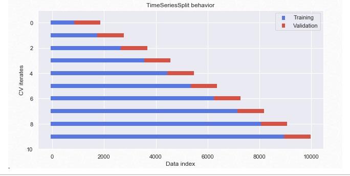
Features and targets datasets split
# Targets dataset:y
y= stations_hourly
# Features dataset:X
X= features_df

# Find the starting indice of the last 10 percent for hold-out datasets
idx= int(len(y)* 0.90)
# Create the features train dataset: X_train
X_train= X.iloc[:idx, :]
# Create the features test dataset: X_test
X_test= X.iloc[idx:, :]
# Create the targets train dataset: y_train
y_train= y.iloc[:idx, :]
# Create the targets test dataset: y_test
y_test= y.iloc[idx: ,:]

print("X_train shape:", X_train.shape, "X_test shape:", X_test.shape)
print("y_train shape:", y_train.shape, "y_test shape:", y_test.shape)
Multi-target models
- Now we have our train and test datasets so we can fit a model and make the predictions. Here we have two approaches:
- 1) to build one model per station
- 2) to predict all the stations together in one model
- One model per station approach is not able to take into account of the similarities between stations.
-
In Sklearn some algorithms like random forest, knn and linear regression natively support multi-target regression thus suitable for second approach
-
The others process the multi-target-regression only with the MultiOutputRegressor but this works as the first approach.
- Here is the explanation from the Sklearn page: "This strategy consists of fitting one regressor per target. This is a simple strategy for extending regressors that do not natively support multi-target regression. As MultiOutputRegressor fits one regressor per target it can not take advantage of correlations between targets.
- Till finding a better solution we will work with the algorithms that natively support multi-target regression
Model with 140 stations
First baseline for the model with 140 stations
-
In this model a target corresponding to a features sample will be a point with the permutations of 140 dimensions(70 arrivals and 70 departures)
-
Here the baseline will be the estimate of these permutations.
- We will take the average of the these permutations i.e hourly arrivals and departures as a baseline for this model and try to beat it.
# Add the time index to stations_hourly df
stations_hourly.index= trips_extended_hourly.index
# Take the averages of the columns
averages= stations_hourly.mean()
# Convert the averages into array
baseline= averages.values
# Stack vertically the baseline to match the y_test shape
baseline= np.tile(averages,(y_test.shape[0], 1))
# Check the shape of baseline
#print("baseline shape:", baseline.shape)

# Baseline errors are the mean of the differences between y_test and the baseline predictions
baseline_error= round (mean_squared_error(y_test.values, baseline)**0.5, 2)
print('Average baseline error: ', baseline_error)
The baseline estimates 1.7 arrivals or departures per hour.
Training the first model
-
Time to build our first model, using random forest implementation from Sklearn.
-
We will use the first 90% of the data for training (the training data set is sorted by time), and the remaining 10% for testing.
-
Let's write a simple function that returns the performance of the model and then train our first regressor.
get_val_score_rf function
- Since we need to calculate model performance during training with tuned parameters it would be better to define a function in order to reuse
def get_val_score_rf(X_tr, y_tr, dct):
    '''
    takes X_train, y_train and a dictionary containing hyperparameter inputs for random forest ->
    returns the cross validation and X_train scores of the model. Both are calculated as
    root mean squared errors
    '''
    # Instantiate a RandomForestRegressor object by unpacking the parameters dictionary
    forest = RandomForestRegressor(**dct)
    # Instantiate TimeSeriesSplit object with 5 splits
    split=TimeSeriesSplit(n_splits=5)
    # Calculate the performance with cross-validation
    score = cross_val_score(forest, X_tr, y_tr, cv=split, scoring='neg_mean_squared_error', n_jobs=-1)
    # Take the sqrt all the splits
    score= np.sqrt(abs(score))
    print("Cross-validation scores:", score,"\n","Cross-validation mean:", f'{np.mean(score):.2f}')
    # fit the model
    forest.fit(X_train, y_train)
    # Predict the train set to see if there is over fitting
    pred_train=forest.predict(X_train)
    print(f'RMSE Train:{np.sqrt(mean_squared_error(y_train, pred_train)):.2f}')
First scores of the model
-
Let's get the first scores of our model with initial hyperparameter settings. We will do the feature selection and hyperparameter tuning afterwards.
-
Let's start with some parameter tips from Sklearn's site to see the first performance.
# Create the params dictionary with basic hyperparameters, include the random_state
initial_params={'n_estimators':100,
        'max_depth':3,
        'min_samples_leaf':2,
        'random_state':37}

# Call the get_val_score_rf on the params dictionary
get_val_score_rf(X_train, y_train, initial_params)
- Model looks little bit underfitting because $rmseTRAIN \approx rmseCV$
- Additional data would be great
-
We can try
- feature selection
- increase the number of estimators, max_depth or decrease min_samples_leaf and look for better combination with other hyperparameters also.
-
We will use this scores as baseline2 and continue to improve our model with feature selection
Feature selection
Feature importance
-
Even though we are using an ensemble method still random forest is dependent on decision trees and decision trees tend to overfit on data with a large number of features
-
We can try omitting the features without prediction power in order to potentially increase the performance of our model and make it computationaly efficient.
-
Let's check the feature importances by using two approach.
- We can get the feature importances from Sklearn RandomForestRegressor however there are other methods also.
-
Here there is an interesting article about the biasedness of the Sklearn Random Forest future importance method.
-
For this work we will try both
Feature importance by sklearn RandomForestRegressor
For regression trees the future importance is measured by how much each feature reduce the variance when they split the data
rf1 = RandomForestRegressor(n_estimators=100, n_jobs=-1)
rf1.fit(X_train, y_train)
# Train the regressor
rf1.predict(X_test)

# Create a pandas Series of features importances: importances
# containing the feature names as index and their importances as values
importances_rf = pd.Series(data=rf1.feature_importances_ , index= X_train.columns)

# Get the sorted importance values: importance_sorted
importance_sorted=importances_rf.sort_values()

# Plot the sorted importance values by using horizontal bars
importance_sorted.plot(kind="barh", color='lightgreen', figsize=(10, 12));

Cumulative importances
- We can get the cumulative importances from the sorted importances and fixed the level that we want to cut off.
- Below the 99% level is drawn for the Sklearn importance ranking
# Sort the importances in descending order
importance_desc=importances_rf.sort_values(ascending=False)
sorted_features=importance_desc.index

# Cumulate the importances
cumulative_importances = np.cumsum(importance_desc)

# list of x locations for plotting
x_values = list(range(len(importance_desc)))

plt.figure(figsize=(14,5))
# Make a line graph
plt.plot(x_values, cumulative_importances, 'g-')
# Draw line at 99% of importance retained
plt.hlines(y = 0.99, xmin=0, xmax=len(importance_desc), color = 'r', linestyles = 'dashed')
# Format x ticks and labels
plt.xticks(x_values, sorted_features, rotation = 'vertical')
# Axis labels and title
plt.xlabel('Variable'); plt.ylabel('Cumulative Importance'); plt.title('Cumulative Importances');

Now we can find number of features for cumulative importance of 99%
# Add 1 because Python is zero-indexed
print('Number of features for 99.5% importance:', np.where(cumulative_importances > 0.995)[0][0] + 1)

# Extract the names of the most important features
important_features = [feature for feature in importance_desc[0:48].index]

# Create training and testing sets with only the important features
X_train_red_sk = X_train[important_features] # red_sk stands for reduced sklearn
X_test_red_sk = X_test[important_features]

# Sanity check
print('Important train features shape:', X_train_red_sk.shape)
print('Important test features shape:', X_test_red_sk.shape)
# Check the scores of the X_train_red_sk to compare with the first feature df X_train
get_val_score_rf(X_train_red_sk, y_train, initial_params)
- After dropping 26 columns from the features dataset we get the same CV mean and RMSE train. It is better to continue with reduced dataset
Feature importance by rfpimp
# Instantiate a random forest object
rf_perm = RandomForestRegressor(n_estimators=100, n_jobs=-1)
# fit the model
rf_perm.fit(X_train, y_train)
# Apply the permutation function
imp = importances(rf_perm, X_test, y_test)
# plot the future importances
viz = plot_importances(imp)
viz.view()
- The results are quite different from each other however in both case as expected the night hours are not predictive.
- In our chart analysis we have seen the bike usage was almost zero between 23h-04h.
- Binary features related with rain are not predictive in both cases, probably the number of the cases are not enough to learn and also it is corelated with humidity
- We can test both of the performances of the two reduced dataset regarding the results of two ranking of importances
Most important futures with rfpimp
# Cumulate the importances
cumulative_imp = np.cumsum(imp.values)
# Add 1 because Python is zero-indexed
print('Number of features for 99.9% importance:', np.where(cumulative_imp > 0.999)[0][0] + 1)

# Extract the names of the most important features
important_perm = [feature for feature in imp[0:20].index]
# Create training and testing sets with only the important features
X_train_perm = X_train[important_perm] # red_sk stands for reduced sklearn
X_test_perm= X_test[important_perm]

# Sanity check
print('Important train features shape:', X_train_perm.shape)
print('Important test features shape:', X_test_perm.shape)
# Check the scores of the X_train_perm to compare with
# the first feature df(X_train) and the X_train_red_sk
get_val_score_rf(X_train_perm, y_train, params)
We get the same score just with 20 columns using rfpimp.
Hyperparameters tuning
Randomized Search CV
- Let's run a randomized search for hyperparameter tuning.
-
We can define a grid of hyperparameter ranges, and randomly sample from the grid by performing cross-validation on each combination of values using Sklearn's
RandomizedSearchCVobject -
Even though RandomizedSearchCV is not an exhaustive search like GridSearch it can be computationally heavy depending on our choise of number of iteration and cross-validation and ranges of hyperparameters.
- Both in Randomized and Grid Search we should use
-
scoring='neg_mean_absolute_error'argument as our loss function is RMSE and -
TimeSeriesSplitas CV splits as we work with timeseries data
-
- Here we will do a simple search with 10 iteration and 2 cross validation and will not tune all the hyperparameters.
# Create the base model to tune
forest_tune = RandomForestRegressor()
# print and see all the parameters of RandomForestRegressor
pprint(forest_tune.get_params())
- As we see there are quite a lot parameters to tune.
- We will focus on the most important ones:
'n_estimators', 'max_depth'and'min_samples_leaf'. - However we will create the full grid to make it ready for furher searches. We can play with the ranges depending on our time.
- Please uncomment the parameters in the dictionary to run a wider search.
# Number of trees in random forest
n_estimators = [int(x) for x in np.linspace(start = 100, stop =1000, num = 3)]
# Number of features to consider at every split
max_features = ['auto', 'sqrt']
# Maximum number of levels in tree
max_depth = [int(x) for x in np.linspace(3, 50, num = 2)]
max_depth.append(None)
# Minimum number of samples required to split a node
min_samples_split = [2, 10]
# Minimum number of samples required at each leaf node
min_samples_leaf = [2, 4]
# Method of selecting samples for training each tree
bootstrap = [True, False]

# Create the random grid
random_grid = {'n_estimators': n_estimators,
               'max_depth': max_depth,
               #'max_features': max_features,
               #'min_samples_split': min_samples_split,
               #'bootstrap': bootstrap
               'min_samples_leaf': min_samples_leaf}

pprint(random_grid)
Since it is not efficient doing random search with the personal laptop at the moment we will try the random search on Google Colab with these parameters.
# Create the splits for timeseries data
split=TimeSeriesSplit(n_splits=2)
# Instantiate a Random Search object with parameters: n_iter = 10, cv = 2,
forest_random = RandomizedSearchCV(estimator = forest_tune,
                                   param_distributions = random_grid,
                                   n_iter = 10,
                                   cv = split,
                                   scoring='neg_mean_absolute_error',
                                   verbose=3,
                                   random_state=37,
                                   n_jobs = -1)

# Fit the random search model on reduced X_train_red_sk
#forest_random.fit(X_train_red_sk, y_train) #(pls uncomment to execute)
First results of the simple randomized search from Colab:

Evaluate random search results
To find out if random search produced better model parameters than the previous one with initial_params we will run with new parameters and compare the results
# Create the best params dictionary
best_params_random={'n_estimators':100,
                    'max_depth':50,
                    'min_samples_leaf':4,
                    'random_state':37}
# Check the scores of the X_train_red_sk
get_val_score_rf(X_train_red_sk, y_train, best_params_random)
Compare the scores before and after search
-
Our first random forest model have the scores:
- Cross-validation mean: 1.23
- RMSE Train:1.23
-
After applying the parameters of randomized search the scores becomes:
- Cross-validation mean: 0.97
- RMSE Train:0.74
The scores are both better and also this time it looks like it does not ovetfit
Grid Search CV
- Random search allowed us to narrow down the range for each hyperparameter.
- Now we can specify more the combination of settings with GridSearchCV
# Create the parameter grid based on the results of random search
param_grid = {'max_depth':[50, 60],
              'min_samples_leaf':[4, 5],
              'n_estimators':[100, 150]}
# Instantiate a RandomForestRegressor object
rf = RandomForestRegressor()
# Instantiate the grid search model
grid_search = GridSearchCV(estimator = rf,
                           param_grid = param_grid,
                           cv = split,
                           scoring='neg_mean_absolute_error',
                           n_jobs = -1,
                           verbose = 2)
pprint(param_grid)
# (pls uncomment to execute)
# Fit the grid search to the data
#grid_search.fit(X_train_red_sk, y_train)
#grid_search.best_params_
First results of the simple grid search from Colab:
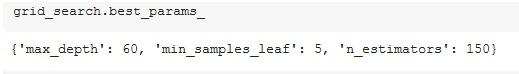
All the parameters augmented little bit.
Evaluate the GridSearch results
# Create the best params dictionary
best_params_grid={'n_estimators':150,
                  'max_depth':60,
                  'min_samples_leaf':5,
                  'random_state':37}
# Check the scores
get_val_score_rf(X_train_red_sk, y_train, best_params_grid)
- Cross-validation mean score did not change. (Only changed in the 3rd decimal probably).
- Train score increased by 0.03 because of maximum depth difference.
- Even though there is chance to improve results by tweaking the ranges.
- For now we can stop our hypermeter tuning here. We will continue to use the previous random search results.
- Again, we have focused only on 3 hyperparameters due to the computational and time constraints.
Hold-out set score
- Now we can see our final test prediction performance by creating our final model
# Instantiate a RandomForestRegressor object with the best parameters of random search
model_rf=RandomForestRegressor(**best_params_random)
# Fit the model
model_rf.fit(X_train_red_sk, y_train)
# Predict the train set
pred_final=model_rf.predict(X_test_red_sk)

print(f'RMSE Test(hold-out):{np.sqrt(mean_squared_error(y_test, pred_final)):.2f}')
- Our test score improved to 0.90 from 0.97 CV mean.
- It is high probaly thanks to the higher amount of training data (we used all the 5 folds together for training)
Test with the reduced X_train_perm
# Instantiate a RandomForestRegressor object with the best parameters of random search
model_rf=RandomForestRegressor(**best_params_random)
# Fit the model
model_rf.fit(X_train_perm, y_train)
# Predict the train set
pred_final=model_rf.predict(X_test_perm)

print(f'RMSE Test(hold-out):{np.sqrt(mean_squared_error(y_test, pred_final)):.2f}')
- We get the same test result by using the features dataset reduced by the
rfpimp - Since
X_train_permhas less columns (20), it looks a better idea to use this dataset for model training and testing.
Reminder:
- So far the model we created predicts the number of arrivals and departures not their differences (net bike stock change)
- Our baselines were also about how close we are to the number of arrivals and departures not the net change.
- To get the net change predictions we need to convert the predictions of the model.
# Save the model for future use
filename = 'model_rf.model'
joblib.dump(model_rf, filename)
# Check if the model properly saved
model=joblib.load(filename)
pred_joblib=model.predict(X_test_perm)
print(f'RMSE Test(hold-out):{np.sqrt(mean_squared_error(y_test, pred_joblib)):.2f}')
-
Our model by construction predicting the number of arrivals and departure seperately thus when we give it unseen data and it returns
[n_unseen_data, 2*stations]matrix. -
So we need to define a function which converts the predictions into net change (
n_departures - n_arrivals)
def net_change(model, df):
    '''
    Takes our model and dataframe to predict returns->
    a dataframe with the half number of columns of the predictons made by our model
    by taking the difference of the departures and arrival columns
    '''
    # Create a dataframe from predictions
    predictions_df = pd.DataFrame(model.predict(df))
    # Create list of column names
    columns_lst = list(predictions_df.columns)
    # Create a list to aggregate the differences of departures and arrivals
    difference_cols =[]
    # Iterate over the column names list till the half point
    for idx in range(len(columns_lst)//2):
        # Collect the column differences in the list
        difference_cols.append(predictions_df[idx+70]-predictions_df[idx])
    # At the end of the loop concat all the columns at once
    net_rate_df = pd.concat(difference_cols, axis=1)
    return net_rate_df
# Call the net_change on our model with test data
net_change(model_rf, X_test_perm).head(2)
As seen above we converted the predictions of arrivals and departures to the differences with 70 columns
Net rates dataframe
- Lets create the net rates dataframe by taking the differences of departures and arrivals for each hour
- In this option the shape will be
[n_hours, n_stations], in our case[8760, 70]
# Create an empty list to aggregate the net change in every row(hour)
columns_lst=[]

## Loop over stations_hourly df columns to find the net change (arrivals-departures)
for station in stations_hourly.columns:
    if station[-1]=="a":
        station_arr = station
        station_dep = station[:-1]+ "d"
        # Append the column difference in the list
        columns_lst.append((stations_hourly[station_arr]- stations_hourly[station_dep]))

# Create the change_df by concatenating the columns in the column_lst
net_df = pd.concat(columns_lst, axis=1)
# Create the column names of the net_df
net_cols =[]
for station in stations_hourly.columns:
    if station[-1]=="a":
        net_cols.append(station[:-1]+ "c")
# Add the column names
net_df.columns = net_cols
net_df.head(2)
net_df.shape
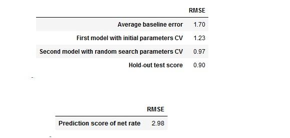
RMSE of the predicted net changes and the actual net changes
Now we can make the final evaluation of our 140 stations approach by finding the RMSE of the prediction of net change and the actual net changes.
# Get the predictions of the test
predicted_net_change= net_change(model_rf, X_test_perm)
# Actual net changes
actual_net_change=y_test_net
# Get the Root Mean Squared Errors of differences
rmse_model_rf=round(mean_squared_error(y_test_net, predicted_net_change)**0.5, 2)
rmse_model_rf
Our model's performance decreased to 2.89 on prediction the net rate change
Target datasets : y_train_net, y_test_net
- We only need to split the targets dataset (
net_df) - We can contunie to use the splitted
X_trainandX_testas features datasets
# Targets dataset:y
y_net= net_df

# Find the starting indice of the last 10 percent for hold-out datasets
idx= int(len(y_net)* 0.90)

# Create the targets train dataset: y_train_net
y_train_net= y_net.iloc[:idx, :]
# Create the targets test dataset: y_test_net
y_test_net= y_net.iloc[idx: ,:]

# Check the shapes
print("X_train shape:", X_train.shape, "X_test shape:", X_test.shape)
print("y_train shape:", y_train_net.shape, "y_test shape:", y_test_net.shape)
First baseline method for net rate approach
# Take the averages of the columns
averages= net_df.mean()
# Convert the averages into array
baseline= averages.values
# Stack vertically the baseline to match the y_test shape
baseline= np.tile(averages,(y_test_net.shape[0], 1))
# Check the shape of baseline
#print("baseline shape:", baseline.shape)
# Baseline errors are the mean of the differences between y_test and the baseline predictions
baseline_error= round (mean_squared_error(y_test_net.values, baseline)**0.5, 2)
print('Average baseline error: ', baseline_error)
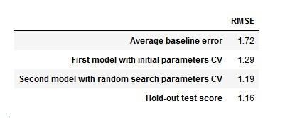
- Quite interesting just taking the daily averages can estimates 1.72 bikes difference on the average
First model performance with net rate targets
We will use the validation function get_val_score_rf that we defined in the previous part to evaluate the first performance of random forest algorithm with the parameters below.
# Create the params dictionary with basic hyperparameters, include the random_state
params={'n_estimators':100,
        'max_depth':3,
        'min_samples_leaf':2,
        'random_state':37}

# Call the get_val_score_rf on X_train_net the params dictionary
get_val_score_rf(X_train, y_train_net, params)
- Even with these parameters net change model beats the first model (140 targets)
- Also these scores are better than the first baseline of this approach
- Score improved from 1.72 to 1.23
Feature importance rfpimp
Now we can continue with the features importance function
# Instantiate a random forest object
rf_perm = RandomForestRegressor(n_estimators=100, n_jobs=-1)
# fit the model
rf_perm.fit(X_train, y_train_net)
# Apply the permutation function
imp = importances(rf_perm, X_test, y_test_net)
# Cumulate the importances
cumulative_imp = np.cumsum(imp.values)
# Add 1 because Python is zero-indexed
print('Number of features for 99.9% importance:', np.where(cumulative_imp > 0.999)[0][0] + 1)
According to model importance funtion only 4 features are enough to get the 99.9% prediction power.
# Extract the names of the most important features. Let's keep 20 of them
important_net = [feature for feature in imp[0:20].index]
# Create training and testing sets with only the important features
X_train_red_net = X_train[important_perm] # red_sk stands for reduced sklearn
X_test_red_net= X_test[important_perm]

# Sanity check
print('Important train features shape:', X_train_red_net.shape)
print('Important test features shape:', X_test_red_net.shape)
Model performance with randomized search parameters
- We did a RandomizedSearchCV on Colab and get the parameters below. Let's get the cross validation scores on reduced features with tweaked parameters
# Parameters from RandomizedSearchCV
params_random={'n_estimators':100,
               'max_depth':50,
               'min_samples_leaf':4,
               'random_state':37}

# Call the get_val_score_rf on X_train_net the params dictionary
get_val_score_rf(X_train_red_net, y_train_net, params_random)
- Cross-validation mean improved from 1.29 to 1.19
- RMSE Train improved from 1.23 to 0.74
Model performance with Grid Search parameters
- After narrowing down the range we ran a simple grid search on Colab to tweak the parameters.
params_grid={'n_estimators':100,
             'max_depth':60,
             'min_samples_leaf':5,
             'random_state':37}

# Call the get_val_score_rf on X_train, y_train_net and the params dictionary
get_val_score_rf(X_train_red_net, y_train_net, params_grid)
- Cross validation score just improved 0.01 and RMSE train get worse 0.03 point. We can use the previous parameters.
Test on hold-out set
- Now we can see our final test prediction performance with net rate targets by creating our final model
# Instantiate a RandomForestRegressor object with the best parameters of random search
model_net_final=RandomForestRegressor(**best_params_random)
# Fit the model
model_net_final.fit(X_train_red_net, y_train_net)
# Predict the train set
pred_final_net=model_net_final.predict(X_test_red_net)

print(f'RMSE Test(hold-out):{np.sqrt(mean_squared_error(y_test_net, pred_final_net)):.2f}')
Our test score on final hold-out set is 1.16 and little better than last cross validation score
Save model for future use 
filename = 'model_net.model'
joblib.dump(model_net_final, filename)
# Check if the model properly saved
model=joblib.load(filename)

pred_joblib=model.predict(X_test_red_net)
print(f'RMSE Test(hold-out):{np.sqrt(mean_squared_error(y_test_net, pred_joblib)):.2f}')
Model with 70 columns targets
- With this final evaluation we completed our steps for this takehome project.
Comments